# Oxla > ## Documentation Index --- # Source: https://docs.oxla.com/sql-reference/sql-functions/math-functions/abs.md > ## Documentation Index > Fetch the complete documentation index at: https://docs.oxla.com/llms.txt > Use this file to discover all available pages before exploring further. # ABS ## Overview The `ABS()` function returns an absolute number, i.e., the positive value of a number. The data type of the returned value will depend on the data type of the value passed to the `ABS()` function. ## Syntax The syntax for the `ABS() `function is as follows: ```sql theme={null} ABS(x) ``` The `ABS()` function requires one argument: * `x`: An expression that evaluates to a number. The **ABS()** function will return the negation of the negative numbers. ## Examples ### Case #1: Absolute value of a negative number The following example demonstrates how the `ABS()` function can be used to obtain the absolute value of a negative number: ```sql theme={null} SELECT ABS(-10.25); ``` It will return an absolute value of the passed argument: ```sql theme={null} +--------+ | f | +--------+ | 10.25 | +--------+ ``` ### Case #2: ABS() function with an expression The following example demonstrates how the `ABS()` function can be used with an expression to obtain the absolute value of the result: ```sql theme={null} SELECT ABS( 100 - 250); ``` The result of the above statement is **-150**. However, you will get the output **150**, as 150 is the positive version of -150. ```sql theme={null} +------+ | f | +------+ | 150 | +------+ ``` ### Case #3: Using the ABS() function with a table The following example demonstrates how the `ABS()` function can be used with a table to obtain the absolute values of all numbers in a specific column: 1. First, create a table named absTable containing an ***initialValue*** column with some positive and negative values: ```sql theme={null} CREATE TABLE absTable(initialValue float); INSERT INTO absTable(initialValue) VALUES (550), (-210), (72.12), (-87.93), (-0.0); ``` 2. Next, use the following query to find the absolute value of all numbers: ```sql theme={null} SELECT initialValue, ABS(initialValue) AS absoluteValue FROM absTable; ``` 3. The above query will retrieve all values in the **"initialValue"** column and their absolute values in the **"absoluteValue"** column. The output will look something like this: ```sql theme={null} +---------------+----------------+ | initialValue | absoluteValue | +---------------+----------------+ | 550 | 550 | | -210 | 210 | | 72.12 | 72.12 | | 87.93 | 87.93 | | -0 | 0 | +---------------+----------------+ ``` --- # Source: https://docs.oxla.com/security/access-control.md > ## Documentation Index > Fetch the complete documentation index at: https://docs.oxla.com/llms.txt > Use this file to discover all available pages before exploring further. # Access Control ## Overview Oxla implements role-based access control (RBAC) features, including roles, privileges and ownership. These features function similarly to those found in other leading database systems, providing a familiar access control model for users and administrators. ## Enabling Access Control Access control is enabled by default on new Oxla installations. You can disable access control through the configuration file if needed. For detailed instructions on configuring access control, refer to the Oxla Configuration File documentation. The access control (AC) behavior is as follows: * If the access control flag is explicitly set in the configuration file, that setting is always followed * If the flag is not explicitly set in the configuration: * When Oxla Home is empty, AC will be **enabled** by default * When Oxla Home is non-empty, AC will be **enabled** only if it was previously enabled For backward compatibility, old Oxla versions did not have access control (AC). If you use a new Oxla release with an Oxla Home created by these old versions, AC will be **disabled** by default. However, if the Oxla Home comes from an older where AC was likely enabled, then AC will be **enabled** by default. This behavior helps maintain security settings appropriate to the Oxla Home’s history. ## Default Superuser Oxla always includes a default superuser account named `oxla` with the initial password `oxla`. * During the first startup, you can set a custom password for the default superuser using the `access_control.initial_password` parameter in the configuration file * After setting the password, you can remove this parameter from the configuration * You can also change the password later using the ALTER ROLE query For security reasons, it is highly recommended to change the default superuser password immediately after installation. ## System Catalogs Visibility Users can view rows in system catalog tables only if those rows correspond to objects or reside in schemas to which the user has access. For example, in the `information_schema.tables` table, a user can see all tables for which they have any grants, as well as all tables in schemas where they have the `USAGE` privilege. ## Restrictions * Only superusers have the `SELECT` privilege on internal system tables * Privileges on internal system tables cannot be granted or revoked * Only superusers and database owners can create new schemas * Only superusers can create new roles * Every role is granted the `CONNECT` privilege to the default database at creation (this privilege can be revoked) * Every role is granted the `USAGE` privilege on the default `public` schema at creation (this privilege can be revoked) * Oxla does not support role membership, so **privilege inheritance** is not available Once access control is enabled and Oxla Home is not empty, you cannot disable access control. If you attempt to run Oxla with the access control flag in `OXLA_HOME` set to `OFF` after it was previously enabled, Oxla will enter a **degraded state**. --- # Source: https://docs.oxla.com/sql-reference/sql-data-types/array.md > ## Documentation Index > Fetch the complete documentation index at: https://docs.oxla.com/llms.txt > Use this file to discover all available pages before exploring further. # Array ## Overview In Oxla, an array allows you to represent a collection of elements that have the same data type (any built-in data type can be used). Currently, the implementation is limited only to single-dimensional arrays ## Array Type Declaration An array type can be declared by appending square brackets to the data type of its elements: ```sql theme={null} CREATE TABLE movie_night ( event_date DATE NOT NULL, movies_planned TEXT[5] NOT NULL ); ``` The syntax above allows you to specify the size of the array. However, it does not enforce any limits and the behavior will be the same for arrays of unspecified length. There is also another way to declare an array, by prepending the `ARRAY` keyword after the data type of the elements: ```sql theme={null} CREATE TABLE movie_night ( event_date DATE NOT NULL, movies_planned TEXT ARRAY NOT NULL ); ``` ## Array Values You can create array literals by using the `ARRAY` keyword and combining it with the array's values enclosed in square brackets and separated by commas: ```sql theme={null} ARRAY[ value1 , value2 , ... ] ``` Such a literal can be used with, e.g. `SELECT` or `INSERT INTO` statements: ```sql theme={null} SELECT ARRAY['10:14:25'::time, '22:58:11'::time]; ?column? --------------------- {10:14:25,22:58:11} (1 row) INSERT INTO movie_night VALUES ('2024-12-01', ARRAY['Inception', 'Interstellar', 'The Prestige']); INSERT 0 1 SELECT * FROM movie_night; event_date | movies_planned ------------+----------------------------------------- 2024-12-01 | {Inception,Interstellar,"The Prestige"} (1 row) ``` You can also use a string representation of an array as another available option for array's values syntax. It requires the elements' values to be enclosed in curly braces and separated by commas: ```sql theme={null} '{ value1 , value2 , ... }' ``` Such an array value representation can be used in e.g. `INSERT INTO` statements with the `VALUES` clause: ```sql theme={null} INSERT INTO movie_night VALUES ('2024-12-15', '{The Matrix, John Wick}'); INSERT 0 1 SELECT * FROM movie_night; event_date | movies_planned ------------+----------------------------------------- 2024-12-01 | {Inception,Interstellar,"The Prestige"} 2024-12-15 | {"The Matrix","John Wick"} (2 rows) ``` Any element can be enclosed in double quotes and this is required, if the value contains commas or curly braces: ```sql theme={null} SELECT '{"{\"key1\": 1, \"key2\": \"value\"}", NULL, true}'::json[]; ?column? ----------------------------------------------- {"{\"key1\":1,\"key2\":\"value\"}",NULL,true} (1 row) ``` In the example above, the double quotes which are a part of the JSON value are required to be escaped with a backslash, so that they are not mistaken with the double quote, which marks the end of the element ## Accessing Arrays You can retrieve a single element from an array using the array subscript operator. When it comes to array values indexing, the elements of an n-length array start at index `1` and end at index `n`: ```sql theme={null} SELECT movies_planned, movies_planned[1] AS first_movie, movies_planned[3] AS third_movie FROM movie_night; movies_planned | first_movie | third_movie -----------------------------------------+-------------+-------------- {Inception,Interstellar,"The Prestige"} | Inception | The Prestige {"The Matrix","John Wick"} | The Matrix | (2 rows) ``` If the index exceeds the length of an array, the returned value will be `NULL` Arrays can also be accessed by using array slices. An array slice is denoted by writing `lower_bound:upper_bound`. The bounds can be omitted, in which case the slice is unbounded from a given side: ```sql theme={null} SELECT movies_planned[:] as "unbounded slice", movies_planned[1:2] AS "[1:2] slice", movies_planned[2:] AS "[2:] slice" FROM movie_night; unbounded slice | [1:2] slice | [2:] slice -----------------------------------------+----------------------------+------------------------------- {Inception,Interstellar,"The Prestige"} | {Inception,Interstellar} | {Interstellar,"The Prestige"} {"The Matrix","John Wick"} | {"The Matrix","John Wick"} | {"John Wick"} (2 rows) ``` ## Limitations ### Field Size Limit In Oxla, the field size limit for variable-size types is 32MB and this limit applies to arrays as well. If a value exceeds the given limit, an error is returned: ```sql theme={null} CREATE TABLE tb (array_column bigint[]); CREATE COPY tb FROM '/.oxla/long_array_value.csv'; ERROR: Error in row 1, column array_column value exceeds size of 33554432 ``` ### Unsupported SQL Clauses Array columns cannot be used as the key columns in `ORDER BY`, `GROUP BY` or `JOIN` operations. It is also impossible to use the array columns as a part of the index of a table. For all the operations mentioned above, an appropriate error message will be returned: ```sql theme={null} SELECT * FROM movie_night ORDER BY movies_planned; ERROR: could not identify an ordering operator for type text[] ``` Arrays can still be used in `ORDER BY` or `JOIN` operations, if the array column is not the key: ```sql theme={null} SELECT * FROM movie_night ORDER BY event_date ASC; event_date | movies_planned ------------+----------------------------------------- 2024-12-01 | {Inception,Interstellar,"The Prestige"} 2024-12-15 | {"The Matrix","John Wick"} (2 rows) ``` ### Unsupported SQL Statements Specific SQL statements currently do not support arrays. These include: * `INSERT INTO` with `SELECT`: Arrays cannot be directly imported using an `INSERT INTO` with a `SELECT` statement. Instead, we encourage you to either use the `COPY FROM CSV` command or the `INSERT INTO` statement with the `VALUES` keyword * `UPDATE` and `DELETE`: Updating or deleting records from a table, which contains array columns is not supported * `COPY TO`: Exporting data from array columns using the `COPY TO` command is not available * `CREATE INDEX`: Index on a table cannot be created on an array column. Any effort to use such operations with arrays will result in an error. For now, these limitations should be considered when designing tables that include array columns. --- # Source: https://docs.oxla.com/sql-reference/sql-functions/window-functions/avg.md # Source: https://docs.oxla.com/sql-reference/sql-functions/aggregate-functions/avg.md > ## Documentation Index > Fetch the complete documentation index at: https://docs.oxla.com/llms.txt > Use this file to discover all available pages before exploring further. # AVG ## Overview The `AVG()` function lets you calculate the average value of records. The input and return types we support can be seen in the table below: | Input type | Return type | | ------------------ | ------------------ | | `INTEGER` | `DOUBLE PRECISION` | | `BIGINT` | `DOUBLE PRECISION` | | `REAL` | `DOUBLE PRECISION` | | `DOUBLE PRECISION` | `DOUBLE PRECISION` | If the input type is 32-bit, then the result will be 64-bit **Special cases:** Returns NaN if the input contains a NaN. ## Examples In this example, we will use an **orders** table that stores details of the purchase transactions: ```sql theme={null} CREATE TABLE orders ( orderid int, custname text, orderproduct text, ordertotal real ); INSERT INTO orders (orderid, custname, orderproduct, ordertotal) VALUES (9557411, 'Maya', 'Jeans', 10.5), (9557421, 'Aaron', 'T-Shirt', 9.2), (9557451, 'Alex', 'Hat', 10.8), (9557311, 'Will', 'Hat', 8.5), (9557321, 'Will', 'T-Shirt', 12.15), (9557351, 'Maya', 'T-Shirt', 9.5), (9557221, 'Maya', 'Jeans', 11.02), (9557251, 'Alex', 'Jeans', 11.09), (9557231, 'Aaron', 'Hat', 14.56), (9557281, 'Aaron', 'Hat', 12.15), (9557291, 'Will', 'T-Shirt', 13.1); ``` ```sql theme={null} SELECT * FROM orders; ``` The above query will show the following table: ```sql theme={null} +----------+-----------+---------------+-------------+ | orderid | custname | orderproduct | ordertotal | +----------+-----------+---------------+-------------+ | 9557411 | Maya | Jeans | 10.5 | | 9557421 | Aaron | T-Shirt | 9.2 | | 9557451 | Alex | Hat | 10.8 | | 9557311 | Will | Hat | 8.5 | | 9557321 | Will | T-Shirt | 12.15 | | 9557351 | Maya | T-Shirt | 9.5 | | 9557221 | Maya | Jeans | 11.02 | | 9557251 | Alex | Jeans | 11.09 | | 9557231 | Aaron | Hat | 14.56 | | 9557281 | Aaron | Hat | 12.15 | | 9557291 | Will | T-Shirt | 13.1 | +----------+-----------+---------------+-------------+ ``` ### AVG() with a single expression In the first example, we want to calculate the average amount of all orders that customers have paid: ```sql theme={null} SELECT AVG(ordertotal) AS "Order Total Average" FROM orders; ``` It will return the following output: ```sql theme={null} +---------------------+ | Order Total Average | +---------------------+ | 11.142727331681685 | +---------------------+ ``` ### AVG() with a GROUP BY clause The following example uses the `AVG()` function and `GROUP BY` clause to calculate the average amount paid by each customer: * First, the `GROUP BY` clause divides orders into groups based on customers * Then, the `AVG` function is applied to each group. ```sql theme={null} SELECT custname AS "Customer", AVG (ordertotal) AS "Total Price Average" FROM orders GROUP BY custname; ``` It will display the output as shown below: ```sql theme={null} +-----------+----------------------+ | Customer | Total Price Average | +-----------+----------------------+ | Aaron | 11.96999994913737 | | Alex | 10.945000171661377 | | Will | 11.25 | | Maya | 10.34000015258789 | +-----------+----------------------+ ``` You can use the cast operator like`::NUMERIC(10,2)` to add two decimal numbers after the comma: ```sql theme={null} SELECT custname AS "Customer", AVG (ordertotal)::NUMERIC(10,2) AS "Total Price Average" FROM orders GROUP BY custname; ``` The result will trim and round two numbers after the comma: ```sql theme={null} +-----------+----------------------+ | Customer | Total Price Average | +-----------+----------------------+ | Aaron | 11.97 | | Alex | 10.95 | | Will | 11.25 | | Maya | 10.34 | +-----------+----------------------+ `` ``` --- # Source: https://docs.oxla.com/sql-reference/sql-functions/math-functions/bitwise-shift-left.md > ## Documentation Index > Fetch the complete documentation index at: https://docs.oxla.com/llms.txt > Use this file to discover all available pages before exploring further. # BITWISE SHIFT LEFT ## Overview Bitwise shift operators in Oxla manipulate the bits of integer value by shifting them left or right. These operations are fundamental in low-level data processing and optimization. The bitwise **left shift (`<<`)** operator shifts the bits of an integer to the left by the specified shift amount. For **integers**, this operation is equivalent to multiplying the integer value by 2 raised to the power of the shift amount. During this operation, high-order bits that are shifted out are permanently lost without the ability to be preserved, while zeros are shifted in from the right to fill the vacant positions. Because the left shifts operation (\<\<) on signed integers is **arithmetic**, meaning it shifts all bits to the left and fills the vacant rightmost bits with zeros on the right, the behavior is the same as a logical shift in this case. However, the overall length of the bit string is preserved, with zeros padding on the right to maintain the length. ## Syntax The syntax for the BITWISE SHIFT LEFT is as follows: ```sql theme={null} value << shift_amount ``` ## Parameters * `value`: integer expression * `shift_amount`: a **non-negative** integer specifying how many bit positions to shift ## Restrictions Bitwise shift operators in Oxla require the shift amount to be a **non-negative** integer. Oxla treats negative shift counts as valid by applying modulo arithmetic based on the bit width, so shifting `1 << -3` in a 32-bit integer is equivalent to shifting `1 << 29`, producing predictable results without errors or undefined behavior. When performing bitwise left shift operations (\<\<) on 32-bit integer values in Oxla, the shift count is taken **modulo** 32. This means: * Shifting by a number of bits greater than or equal to 32 will wrap around * For example, `1 << 35` is equivalent to `1 << 3` because `35`$modulo$`32 = 3` If you shift by a value larger than or equal to 32, the actual shift will be the remainder after dividing by 32, which may lead to unexpected results if not carefully considered. ## Examples For the needs of this section we will use a simplified version of the `film` table from the Pagila database, containing only the `title`, `rating` and `privilegs` columns. The complete schema for the `film` table can be found on the Pagila database website. ```sql theme={null} DROP TABLE IF EXISTS film; CREATE TABLE film ( title TEXT NOT NULL, rating TEXT, privileges INT NOT NULL ); INSERT INTO film(title, rating, privileges) VALUES ('ATTRACTION NEWTON', 'PG-13', 1), -- Free users ('CHRISTMAS MOONSHINE', 'NC-17', 2), -- Premium users ('DANGEROUS UPTOWN', 'PG', 3), -- Free + Premium users (bits 0 and 1) ('KILL BROTHERHOOD', 'G', 4), -- Admin-only content ('HALLOWEEN NUTS', 'PG-13', 1), ('HOURS RAGE', 'NC-17', 2), ('PIANIST OUTFIELD', 'NC-17', 3), ('PICKUP DRIVING', 'G', 4), ('INDEPENDENCE HOTEL', 'NC-17', 1), ('PRIVATE DROP', 'PG', 2), ('SAINTS BRIDE', 'G', 3), ('FOREVER CANDIDATE', 'NC-17', 4), ('MILLION ACE', 'PG-13', 1), ('SLEEPY JAPANESE', 'PG', 2), ('WRATH MILE', 'NC-17', 3), ('YOUTH KICK', 'NC-17', 4), ('CLOCKWORK PARADISE', 'PG-13', 1); ``` * Privilege 1 (binary 0001): Free users can watch. * Privilege 2 (binary 0010): Premium users can watch. * Privilege 3 (binary 0011): Both free and premium users can watch. * Privilege 4 (binary 0100): Admin-only content. The query below uses the integer `Left shift (<<)` operation, shifting the privileges value left by 1 for the movie 'ATTRACTION NEWTON': ```sql theme={null} UPDATE film SET privileges = privileges << 1 WHERE title = 'ATTRACTION NEWTON'; ``` After running the update, you can verify the change with: ```sql theme={null} SELECT title, privileges FROM film WHERE title = 'ATTRACTION NEWTON'; ``` Expected output: ```sql theme={null} title | privileges -------------------+------------ ATTRACTION NEWTON | 2 (1 row) ``` --- # Source: https://docs.oxla.com/sql-reference/sql-functions/math-functions/bitwise-shift-right.md > ## Documentation Index > Fetch the complete documentation index at: https://docs.oxla.com/llms.txt > Use this file to discover all available pages before exploring further. # BITWISE SHIFT RIGHT Bitwise shift operators in Oxla manipulate the bits of integer value by shifting them left or right. These operations are fundamental in low-level data processing and optimization. The bitwise **right shift (`>>`)** operator shifts the bits of an integer to the right by the specified number of positions. For **integers**, this operation is equivalent to dividing the integer value by 2 raised to the power of the shift amount, discarding any remainder. Unlike a logical shift, the right shift in Oxla is an **arithmetic** shift, meaning that the vacant leftmost bits are filled with the original sign bits (the most significant bit) rather than zeros. This preserves the sign of the integer after the shift, ensuring correct behavior for signed values. During the shift, low-order bits that move beyond the size limit are permanently lost. However, the overall length of the bit string is preserved, with zeros padding on the left side to maintain the length. ## Syntax The syntax for the BITWISE SHIFT RIGHT is as follows: ```sql theme={null} value >> shift_amount ``` ## Parameters * `value`: integer expression * `shift_amount`: a **non-negative** integer specifying how many bit positions to shift ## Restrictions Bitwise shift operators in Oxla require the shift amount to be a **non-negative** integer. Oxla treats negative shift counts as valid by applying modulo arithmetic based on the bit width, so shifting `1 >> -3` in a 32-bit integer is equivalent to shifting `1 >> 29`, producing predictable results without errors or undefined behavior. When performing bitwise right shift operations (>>) on 32-bit integer values in Oxla, the shift count is taken **modulo** 32, just as with left shifts. This means: * Shifting by a number of bits greater than or equal to 32 will wrap around * For example `1 >> 35` is equivalent to `1 >> 3` because `35`$modulo$`32 = 3` If you shift by a value larger than or equal to 32, the actual shift will be the remainder after dividing by 32, which may lead to unexpected results if not carefully considered. ## Examples For the needs of this section we will use a simplified version of the `film` table from the Pagila database, containing only the `title`, `rating` and `privilegs` columns. The complete schema for the `film` table can be found on the Pagila database website. ```sql theme={null} DROP TABLE IF EXISTS film; CREATE TABLE film ( title TEXT NOT NULL, rating TEXT, privileges INT NOT NULL ); INSERT INTO film(title, rating, privileges) VALUES ('ATTRACTION NEWTON', 'PG-13', 1), -- Free users ('CHRISTMAS MOONSHINE', 'NC-17', 2), -- Premium users ('DANGEROUS UPTOWN', 'PG', 3), -- Free + Premium users (bits 0 and 1) ('KILL BROTHERHOOD', 'G', 4), -- Admin-only content ('HALLOWEEN NUTS', 'PG-13', 1), ('HOURS RAGE', 'NC-17', 2), ('PIANIST OUTFIELD', 'NC-17', 3), ('PICKUP DRIVING', 'G', 4), ('INDEPENDENCE HOTEL', 'NC-17', 1), ('PRIVATE DROP', 'PG', 2), ('SAINTS BRIDE', 'G', 3), ('FOREVER CANDIDATE', 'NC-17', 4), ('MILLION ACE', 'PG-13', 1), ('SLEEPY JAPANESE', 'PG', 2), ('WRATH MILE', 'NC-17', 3), ('YOUTH KICK', 'NC-17', 4), ('CLOCKWORK PARADISE', 'PG-13', 1); ``` * Privilege 1 (binary 0001): Free users can watch. * Privilege 2 (binary 0010): Premium users can watch. * Privilege 3 (binary 0011): Both free and premium users can watch. * Privilege 4 (binary 0100): Admin-only content. The query below uses the integer `right shift (>>)` operation, shifting the privileges value right by 1 for the movie 'DANGEROUS UPTOWN': ```sql theme={null} UPDATE film SET privileges = privileges >> 1 WHERE title = 'DANGEROUS UPTOWN'; ``` After running the update, you can verify the change with: ```sql theme={null} SELECT title, privileges FROM film WHERE title = 'DANGEROUS UPTOWN'; ``` Expected output: ```sql theme={null} title | privileges -------------------+------------ DANGEROUS UPTOWN | 1 (1 row) ``` --- # Source: https://docs.oxla.com/sql-reference/sql-functions/window-functions/bool-and.md # Source: https://docs.oxla.com/sql-reference/sql-functions/aggregate-functions/bool-and.md > ## Documentation Index > Fetch the complete documentation index at: https://docs.oxla.com/llms.txt > Use this file to discover all available pages before exploring further. # BOOL_AND ## Overview The `BOOL_AND()` function calculates all the boolean values in the aggregated group, which will have these results: * `true` if all the values are `true` for every row. * `false` if at least one row in the group is `false`. The input and the return type must be in `BOOL`. `NULL` values are not aggregated, so it will return `NULL` if there are zero input rows. ## Examples In this example, we will use a payment table that stores details of the orders, whether the order has been paid or unpaid by the customer: ```sql theme={null} CREATE TABLE payment ( orderid int, custname text, orderproduct text, ordertotal real, paid boolean ); INSERT INTO payment (orderid, custname, orderproduct, ordertotal, paid) VALUES (9557411, 'Maya', 'Jeans', 10.5, true), (9557421, 'Aaron', 'T-Shirt', 9.2, true), (9557451, 'Alex', 'Hat', 10.8, true), (9557311, 'Will', 'Hat', 8.5, true), (9557321, 'Will', 'T-Shirt', 12.15, true), (9557351, 'Maya', 'T-Shirt', 9.5, true), (9557221, 'Maya', 'Jeans', 11.02, true), (9557251, 'Alex', 'Jeans', 11.09, true), (9557231, 'Aaron', 'Hat', 14.56, false), (9557281, 'Aaron', 'Hat', 12.15, true), (9557291, 'Will', 'T-Shirt', 13.1, true); ``` ```sql theme={null} SELECT * FROM payment; ``` The above query will show the following table: ```sql theme={null} +----------+-----------+---------------+-------------+-------+ | orderid | custname | orderproduct | ordertotal | paid | +----------+-----------+---------------+-------------+-------+ | 9557411 | Maya | Jeans | 10.5 | t | | 9557421 | Aaron | T-Shirt | 9.2 | t | | 9557451 | Alex | Hat | 10.8 | t | | 9557311 | Will | Hat | 8.5 | t | | 9557321 | Will | T-Shirt | 12.15 | t | | 9557351 | Maya | T-Shirt | 9.5 | t | | 9557221 | Maya | Jeans | 11.02 | t | | 9557251 | Alex | Jeans | 11.09 | t | | 9557231 | Aaron | Hat | 14.56 | f | | 9557281 | Aaron | Hat | 12.15 | t | | 9557291 | Will | T-Shirt | 13.1 | t | +----------+-----------+---------------+-------------+-------+ ``` ### Case #1: `BOOL_AND` with a false result We will find out if all customers have paid for their orders using the query below: ```sql theme={null} SELECT BOOL_AND(paid) AS "final_result" FROM payment; ``` In the `BOOL_AND` function, if there is at least one `FALSE` value, the overall result will be `FALSE`. The final output shows that there is an order that hasn’t been paid. ```sql theme={null} +--------------+ | final_result | +--------------+ | f | +--------------+ ``` ### Case #2: `BOOL_AND` with a true result We will find out if Maya has paid for her orders using the query below: ```sql theme={null} SELECT BOOL_AND(paid) AS Maya_Paid FROM payment WHERE custname ='Maya'; ``` In the `BOOL_AND` function, if all values are `TRUE`, then the overall result will be `TRUE`. The final output shows that Maya has paid all her orders. ```sql theme={null} +------------+ | maya_paid | +------------+ | t | +------------+ ``` --- # Source: https://docs.oxla.com/sql-reference/sql-functions/window-functions/bool-or.md # Source: https://docs.oxla.com/sql-reference/sql-functions/aggregate-functions/bool-or.md > ## Documentation Index > Fetch the complete documentation index at: https://docs.oxla.com/llms.txt > Use this file to discover all available pages before exploring further. # BOOL_OR ## Overview The `BOOL_OR()` function calculates all the boolean values in the aggregated group, which will have these results: * `false` if all the values are `false` for every row. * `true` if at least one row in the group is true. The input and the return type must be in `BOOL`. `NULL` values are not aggregated, so it will return `NULL` if there are zero input rows. ## Examples In this example, we will use a payment\*\* \*\*table that stores details of the orders, whether the order has been paid or unpaid by the customer: ```sql theme={null} CREATE TABLE payment ( orderid int, custname text, orderproduct text, ordertotal real, paid boolean ); INSERT INTO payment (orderid, custname, orderproduct, ordertotal, paid) VALUES (9557411, 'Maya', 'Jeans', 10.5, false), (9557421, 'Aaron', 'T-Shirt', 9.2, false), (9557451, 'Alex', 'Hat', 10.8, false), (9557311, 'Will', 'Hat', 8.5, true), (9557321, 'Will', 'T-Shirt', 12.15, false), (9557351, 'Maya', 'T-Shirt', 9.5, true), (9557221, 'Maya', 'Jeans', 11.02, false), (9557251, 'Alex', 'Jeans', 11.09, false), (9557231, 'Aaron', 'Hat', 14.56, false), (9557281, 'Aaron', 'Hat', 12.15, false), (9557291, 'Will', 'T-Shirt', 13.1, false); ``` ```sql theme={null} SELECT * FROM payment; ``` The above query will show the following table: ```sql theme={null} +----------+-----------+---------------+-------------+--------+ | orderid | custname | orderproduct | ordertotal | paid | +----------+-----------+---------------+-------------+--------+ | 9557411 | Maya | Jeans | 10.5 | f | | 9557421 | Aaron | T-Shirt | 9.2 | f | | 9557451 | Alex | Hat | 10.8 | f | | 9557311 | Will | Hat | 8.5 | t | | 9557321 | Will | T-Shirt | 12.15 | f | | 9557351 | Maya | T-Shirt | 9.5 | t | | 9557221 | Maya | Jeans | 11.02 | f | | 9557251 | Alex | Jeans | 11.09 | f | | 9557231 | Aaron | Hat | 14.56 | f | | 9557281 | Aaron | Hat | 12.15 | f | | 9557291 | Will | T-Shirt | 13.1 | f | +----------+-----------+---------------+-------------+--------+ ``` ### Case #1: `BOOL_OR` with a true result We will find out if all customers have paid for their orders using the query below: ```sql theme={null} SELECT BOOL_OR(paid) AS "final_result" FROM payment; ``` If there is at least one `TRUE` value, the overall result will be `TRUE`. The final output shows that some order has been paid regardless of the other unpaid orders. ```sql theme={null} +--------------+ | final_result | +--------------+ | t | +--------------+ ``` ### Case #2: `BOOL_OR` with a false result We will find out if Aaron has paid for his orders using the query below: ```sql theme={null} SELECT BOOL_OR(paid) AS aaron_paid FROM payment WHERE custname ='Aaron'; ``` If all values are `FALSE`, then the overall result will be `FALSE`. The final output shows that Aaron hasn’t paid for all his orders. ```sql theme={null} +-------------+ | aaron_paid | +-------------+ | f | +-------------+ ``` --- # Source: https://docs.oxla.com/sql-reference/sql-data-types/bool.md > ## Documentation Index > Fetch the complete documentation index at: https://docs.oxla.com/llms.txt > Use this file to discover all available pages before exploring further. # Bool ## **Overview** A `BOOL` is a data type mainly used for expressions that will return only two possible values, `true` and `false`. Bool is stored as a bitmap in `u64` values. **BOOLEAN** is an alias for the **BOOL** data type. You can create a table using **BOOLEAN**. However, it will be stored and processed equivalently to **BOOL**. ## Format * `FALSE` * `TRUE` ## **Examples** Below are a few examples of using a bool data type: ### Case #1: Create a Table A librarian will create a **borrowBook** table that he will use to store book borrowing data. The table comprises the borrowed ID, the book name, the borrower, and the book's returned status, which uses the **bool** data type. ```sql theme={null} CREATE TABLE borrowBook ( borrowID INT, bookName TEXT, borrower TEXT, returnedStat BOOL NOT NULL ); INSERT INTO borrowBook (borrowID,bookName, borrower, returnedStat) VALUES (101, 'The Silent Patient', 'Mike', TRUE), (201, 'Malibu Rising', 'Jean', TRUE), (301, 'The Guest List', 'Mark', FALSE), (401, 'The Four Winds', 'Cliff', TRUE), (501, 'The Vanishing Half: A Novel', 'Sarah', TRUE), (601, 'Red, White & Royal Blue', 'Anna', FALSE), (701, 'The Duke and I', 'Blake', FALSE), (801, 'The Lord of the Rings', 'Sandra', FALSE); ``` The **borrowBook** table has been successfully created after executing the above query: ```sql theme={null} COMPLETE INSERT 0 8 ``` ### Case #2: Display the Table Run the `SELECT` statement to get all records from the **borrowBook** table: ```sql theme={null} SELECT * FROM borrowBook; ``` It will return the result as displayed below: ```sql theme={null} +-----------+---------------------------------+------------+---------------+ | borrowid | bookname | borrower | returnedstat | +-----------+---------------------------------+------------+---------------+ | 101 | The Silent Patient | Mike | t | | 201 | Malibu Rising | Jean | t | | 301 | The Guest List | Mark | f | | 401 | The Four Winds | Cliff | t | | 501 | The Vanishing Half: A Novel | Sarah | t | | 601 | Red, White & Royal Blue | Anna | f | | 701 | The Duke and I | Blake | f | | 801 | The Lord of the Rings | Sandra | f | +-----------+---------------------------------+------------+---------------+ ``` ### Case #3: List of the Returned Books In the below example, the following statement is used to retrieve all the **books** that have already been returned: ```sql theme={null} SELECT * FROM borrowbook WHERE returnedstat= 'true'; ``` We will get the following results: ```sql theme={null} +-----------+---------------------------------+------------+---------------+ | borrowid | bookname | borrower | returnedstat | +-----------+---------------------------------+------------+---------------+ | 101 | The Silent Patient | Mike | t | | 201 | Malibu Rising | Jean | t | | 401 | The Four Winds | Cliff | t | | 501 | The Vanishing Half: A Novel | Sarah | t | +-----------+---------------------------------+------------+---------------+ ``` ### Case #4: List of the Unreturned Books Now, we will acquire all of the book records that haven’t been returned yet by running the `SELECT` statement with a specified `WHERE` condition as `false`: ```sql theme={null} SELECT * FROM borrowbook WHERE returnedstat= 'false'; ``` We will get the following results: ```sql theme={null} +-----------+---------------------------------+------------+---------------+ | borrowid | bookname | borrower | returnedstat | +-----------+---------------------------------+------------+---------------+ | 301 | The Guest List | Mark | f | | 601 | Red, White & Royal Blue | Anna | f | | 701 | The Duke and I | Blake | f | | 801 | The Lord of the Rings | Sandra | f | +-----------+---------------------------------+------------+---------------+ ``` ### Case #5: Check a Book’s Return Status In this example, we are going to figure out the returned status of the book **“The Lord of the Rings”** by executing the `SELECT` statement with a specified column in the `WHERE` clause: ```sql theme={null} SELECT * FROM borrowbook WHERE bookname = 'The Lord of the Rings'; ``` The above query will filter all records based on the specified conditions, and we know that Sandra hasn’t returned the book yet: ```sql theme={null} +-----------+---------------------------------+------------+---------------+ | borrowid | bookname | borrower | returnedstat | +-----------+---------------------------------+------------+---------------+ | 801 | The Lord of the Rings | Sandra | f | +-----------+---------------------------------+------------+---------------+ ``` --- # Source: https://docs.oxla.com/sql-reference/sql-functions/math-functions/cbrt.md > ## Documentation Index > Fetch the complete documentation index at: https://docs.oxla.com/llms.txt > Use this file to discover all available pages before exploring further. # CBRT ## Overview The `CBRT()` function calculates and returns the cube root of a given number. In mathematical terms, for a number *x*, its cube root *y* is determined by the equation *y³ = x*. ## Syntax The syntax for the `CBRT()` function is as follows: ```sql theme={null} CBRT(number) ``` Where: * `number`: This is a required value representing the number for which you want to calculate the cube root. It can be a positive or negative whole number, a decimal, or even an expression that evaluates to a number. For example, you can use expressions like `SELECT CBRT(some_column) from test_table`, assuming `some_column` contains a numeric value. **Return Value:**
- It will return `NULL` if the argument is `NULL`.
- It will give an error if you input a parameter that is not a numeric type.
## Examples Below are several usage examples of the `CBRT()` function: ### Case #1: **Basic Cube Root Calculation** Consider the following example: ```sql theme={null} SELECT CBRT(125); ``` The result of this query will be: ```sql theme={null} cbrt ------ 5 ``` ### Case #2: **Cube Root of a Negative Value** To calculate the cube root of a negative number, use the `CBRT()` function as shown: ```sql theme={null} SELECT CBRT(-125); ``` The final result is as follows. ```sql theme={null} cbrt ------ -5 ``` ### Case #3: **Cube Root of Decimal Result** For calculations with decimal numbers, use the `CBRT()` function as demonstrated below: ```sql theme={null} SELECT CBRT(32); ``` The result will be a decimal value, as shown below: ```sql theme={null} cbrt ------------------- 3.174802103936399 ``` ### Case #4: **Cube Root of Decimal Input** In this scenario, fractional seconds are incorporated into the argument: ```sql theme={null} SELECT CBRT(0.12815); ``` The result will be the cube root of the provided decimal value. ```sql theme={null} cbrt ------------ 0.50416523 ``` ### Case #5: Handling Incorrect Argument When a non-numeric argument is provided, the `CBRT()` function works as follows: ```sql theme={null} SELECT CBRT('abc'); ``` An error will be generated, and the result will not be valid. ```sql theme={null} invalid input syntax for type double precision: "abc" ``` ### Case #6: CBRT Operator (`||/(x)`) Here's an example using the CBRT operator (`||/(x)`) to calculate the cube root of a given number: ```sql theme={null} SELECT ||/(1728) AS cbrt_operator; ``` In this example, we calculate the cube root of 1728 using the CBRT operator. The result of this query will be: ```sql theme={null} cbrt_operator -------------------- 12.000000000000002 ``` --- # Source: https://docs.oxla.com/sql-reference/sql-functions/math-functions/ceil.md > ## Documentation Index > Fetch the complete documentation index at: https://docs.oxla.com/llms.txt > Use this file to discover all available pages before exploring further. # CEIL ## Overview The `CEIL()` function returns the nearest positive or negative integer value greater than or equal to the provided decimal input number. ## Syntax The syntax of the `CEIL()` function is as follows: ```sql theme={null} CEIL(x) ``` The `CEIL()` function requires one argument: * `x`: A positive or a negative decimal number (or an expression that evaluates to a decimal number). ## Examples ### Case #1: Rounding up a positive decimal value The following example demonstrates how the `CEIL() `function rounds up a positive decimal value: ```sql theme={null} SELECT CEIL (300.55); ``` As shown below, it will return 301, as it is the nearest integer value greater than 300.55. ```sql theme={null} +------+ | f | +------+ | 301 | +------+ ``` ### Case #2: Rounding up a negative decimal value The following example demonstrates how the `CEIL() `function rounds up a negative decimal value: ```sql theme={null} SELECT CEIL(-89.9) AS "Ceil"; ``` The output of this statement will be -89, as -89 is the nearest integer value greater than or equal to -89.9, as shown below. ```sql theme={null} +-------+ | Ceil | +-------+ | -89 | +-------+ ``` ### Case #3: Using the `CEIL()` function with a table The following example demonstrates how the `CEIL()` function can be used with a table to round up the values in a specific column: 1. First, create a table called ***CeilRecords*** with the following query: ```sql theme={null} CREATE TABLE CeilRecords (numbers float); INSERT INTO CeilRecords(numbers) VALUES (-28.85), (-9.4), (0.87), (78.16), (42.16); ``` The above statement will create a table called **"CeilRecords"** with a column called **"numbers"** and insert 5 decimal values into it. 2. The statement below can be used to retrieve and round up the value for all records in the column \***numbers**: ```sql theme={null} SELECT *, CEIL(numbers) AS CeilValue FROM CeilRecords; ``` The final result will contain the following: * A **numbers** column with initial decimal values. * A **CeilValue** column with rounded-up integer values. ```sql theme={null} +---------+------------+ | numbers | CeilValue | +---------+------------+ | -28.85 | -28 | | -9.4 | -9 | | 0.87 | 1 | | 78.16 | 79 | | 42.16 | 43 | +---------+------------+ ``` --- # Source: https://docs.oxla.com/sql-reference/sql-functions/other-functions/coalesce.md > ## Documentation Index > Fetch the complete documentation index at: https://docs.oxla.com/llms.txt > Use this file to discover all available pages before exploring further. # coalesce() ## Overview Tables can hold null and non-null values. Yet, often we prefer to overlook those null values and this is where `COALESCE()` steps in. It helps when we want to ignore null values while processing the data, by returning the first argument that is not null, while the remaining arguments from the first non-null argument are not evaluated. If all arguments are null, the COALESCE function will return null. ## Syntax The syntax for the `COALESCE()` function is as follows: ```sql theme={null} COALESCE (argument_1, argument_2, …); ``` Key points from the syntax: * `COALESCE()` requires a minimum of two inputs. * It can take an unlimited number of arguments. * Evaluation occurs sequentially from left to right, stopping at the first non-null value. ## Examples Here are some examples to illustrate the application of `COALESCE()`: ### Case #1: Returning the First Non-Null Value In this example, we have a set of values. By using the `COALESCE()` function, we're going to get the first non-null value from this set. ```sql theme={null} SELECT COALESCE(9, 3, 8, 7, 1); ``` The result will be `9`, the first value without null among the provided options. ```sql theme={null} coalesce ---------- 9 ``` ### Case #2: Handling NULL Value as the Last Argument Let's include NULL as the final argument and check the query output. ```sql theme={null} Select COALESCE(3,4,5,9,10,NULL); ``` The function output is `3` because it returns the first non-null value. ```sql theme={null} coalesce ---------- 3 ``` ### Case #3: Handling NULL Value as the First Argument Consider NULL as the first argument in the following example. ```sql theme={null} Select COALESCE(NULL,1,5,7,9,2); ``` The output is `1`, as it is the first non-null value of the argument. ```sql theme={null} coalesce ---------- 1 ``` ### Case #4: Handling Multiple NULL Values In the following query, NULL appears in the first, second, fourth, and last positions. ```sql theme={null} Select COALESCE(NULL, NULL ,3, NULL, 7,9,4,5, NULL); ``` The `COALESCE()` function ignores the first two NULLs and returns the first non-null value, `3`. It does not process the subsequent NULL values. ```sql theme={null} coalesce ---------- 3 ``` ### Case #5: Handling All NULL Values Assume that the given values are entirely composed of nulls. ```sql theme={null} Select COALESCE(NULL, NULL ,NULL, NULL); ``` In this case, the `COALESCE()` function returns an empty value (null). ```sql theme={null} coalesce ---------- ``` ### Case #6: `COALESCE()` with Table Data Imagine we have the `employee_absent` table, which comprises a mix of NULL and non-null values: ```sql theme={null} CREATE TABLE employee_absent ( emp_name TEXT, emp_dept TEXT, absent TEXT ); INSERT INTO employee_absent (emp_name, emp_dept, absent) VALUES ('Alice', 'Finance', 'absent'), ('Bob', 'Operations', 'absent'), ('Carol', 'Finance', 'absent'), ('David', 'HR', NULL), ('Emily', 'HR', NULL); ``` Use the `SELECT` statement to display all the records: ```sql theme={null} SELECT * FROM employee_absent; ``` ```sql theme={null} emp_name | emp_dept | absent ----------+------------+-------- Alice | Finance | absent Bob | Operations | absent Carol | Finance | absent David | HR | Emily | HR | ``` The query below uses the `COALESCE()` function on the `absent` column. It retrieves names and absences (with `out of office` for NULL values) for each employee. ```sql theme={null} SELECT emp_name, COALESCE(absent, 'out of office') AS DisplayAbsent FROM employee_absent; ``` ```sql theme={null} emp_name | displayabsent ----------+--------------- Alice | absent Bob | absent Carol | absent David | out of office Emily | out of office ``` ### Case #7: Error Output in `COALESCE()` When specifying arguments with different datatypes, they should be convertible. ```sql theme={null} Select Coalesce ('x',NULL,1); ``` If the datatypes cannot be converted, the `COALESCE()` function will generate an error, as shown below. ```sql theme={null} ERROR: invalid input syntax for type integer: "x" ``` --- # Source: https://docs.oxla.com/sql-reference/sql-functions/other-functions/col-description.md > ## Documentation Index > Fetch the complete documentation index at: https://docs.oxla.com/llms.txt > Use this file to discover all available pages before exploring further. # col_description() ## Overview The col\_description() is a comment information function that retrieves the comment associated with a specified table column. ## Syntax The syntax for the `col_description()` function is as follows:
col\_description (table\_oid, column\_number) → NULL
## Parameters The following parameters are required to execute this function: * table\_oid: specifies the object identifier (OID) of the table containing the column for which you want to retrieve the comment * column\_number: indicates the ordinal position of the column within the table (starting from 1 for the first column) It is important to note that the column number must be provided as an object identifier (OID), which can be achieved by casting the table name to `regclass` ## Restrictions * This function always returns `NULL` if there are no parameters specified --- # Source: https://docs.oxla.com/sql-reference/comment-support.md > ## Documentation Index > Fetch the complete documentation index at: https://docs.oxla.com/llms.txt > Use this file to discover all available pages before exploring further. # Comment Support ## Overview OXLA fully supports comments in your queries. Comments provide a way to add explanatory notes and improve the readability of queries, making it easier for developers and stakeholders to understand complex queries. There are two types of comments in OXLA: **single-line** and **multi-line (block)**. ## Single Line Comments A single-line comment in OXLA starts with two consecutive hyphens (--) and extends to the end of the line. These comments are used to annotate specific parts of a query, providing brief explanations or notes to assist in understanding the query. **Syntax:** ```sql theme={null} -- This is an example single line comment ``` ## Multi-Line (Block) Comments OXLA also supports multi-line comments, often referred to as block comments. These comments begin with /\* and end with \*/, allowing for multi-line explanations or temporarily disabling sections of the query. **Syntax:** ```sql theme={null} /* This is an example multi-line comment. It can span multiple lines and is useful for providing detailed explanations. */ ``` ## Comment Placement In OXLA, single-line comments should always be placed at the end of the line they refer to, whereas multi-line comments can be positioned anywhere within the query. **Example - Comment on Single Line:** ```sql theme={null} SELECT column1, column2 -- This is an example single line comment FROM table_name; ``` **Example - Comment on Multiple Lines:** ```sql theme={null} SELECT /* comment 1 */ column1, column2 FROM table_name /* comment 2 */ WHERE column3 = 42 /* comment 3 */ ; ``` ## Best Practices for Commenting To maximize the benefits of comments in OXLA queries, follow these best practices: Write clear and concise comments that provide meaningful insights into the specific parts of the query. Whenever the query is modified, update the associated comments to reflect the changes accurately. While comments are helpful, excessive commenting can clutter the code and reduce. --- # Source: https://docs.oxla.com/sql-reference/sql-functions/string-functions/concat.md > ## Documentation Index > Fetch the complete documentation index at: https://docs.oxla.com/llms.txt > Use this file to discover all available pages before exploring further. # CONCAT ## Overview The `CONCAT()` function is used to concatenate one or more input values into a single result. It supports all data types in Oxla, except `TIMESTAMPTZ`, and the output will be returned as a concatenation of the input values. **Special cases:** Returns `NULL` if there are no input rows or `NULL` values. ## Examples ### Case 1: Basic `CONCAT()` function The below example uses the `CONCAT()` function to concatenate three values = into a single result: ```sql theme={null} SELECT CONCAT ('Oxla', '.', 'com') AS "Website"; ``` The final result will be as follows: ```sql theme={null} +------------+ | Website | +------------+ | Oxla.com | +------------+ ``` ### Case 2: `CONCAT()` function using column We have an example of a **payment** table that stores customer payment data. ```sql theme={null} CREATE TABLE payment ( paymentid int, custFirstName text, custLastName text, product text, ordertotal int ); INSERT INTO payment (paymentid, custFirstName, custLastName, product, ordertotal) VALUES (9557451,'Alex','Drue','Latte',2.10), (9557421,'Lana','Rey','Latte',2.10), (9557411,'Tom','Hanks','Americano',1.85), (9557351,'Maya','Taylor','Cappuccino',2.45), (9557321,'Smith','Jay','Cappuccino',2.45), (9557311,'Will','Ritchie','Americano',1.85); ``` ```sql theme={null} SELECT * FROM payment; ``` The above query will display the following table: ```sql theme={null} +------------+----------------+----------------+--------------+---------------+ | paymentid | custFirstName | custLastName | product | ordertotal | +------------+----------------+----------------+--------------+---------------+ | 9557451 | Alex | Drue | Latte | 2.10 | | 9557421 | Lana | Rey | Latte | 2.10 | | 9557411 | Tom | Hanks | Americano | 1.85 | | 9557351 | Maya | Taylor | Cappuccino | 2.45 | | 9557321 | Smith | Jay | Cappuccino | 2.45 | | 9557311 | Will | Ritchie | Americano | 1.85 | +------------+----------------+----------------+--------------+---------------+ ``` The following query will concatenate values in the `custFirstName` and `custLastName` columns of the **payment** table: ```sql theme={null} SELECT CONCAT (custFirstName, ' ', custLastName) AS "Customer Name" FROM payment; ``` It will display an output where spaces separate the first and last names. ```sql theme={null} +-----------------+ | Customer Name | +-----------------+ | Tom Hanks | | Lana Rey | | Alex Drue | | Will Ritchie | | Smith Jay | | Maya Taylor | +-----------------+ ``` ### Case 3: CONCAT() function with NULL We use the `CONCAT()` function in the following example to concatenate a string with a `NULL` value: ```sql theme={null} SELECT CONCAT('Talent Source ',NULL) AS "concat"; ``` The result shows that the `CONCAT` function will skip the `NULL` value: ```sql theme={null} +------------------+ | concat | +------------------+ | Talent Source | +------------------+ ``` --- # Source: https://docs.oxla.com/sql-reference/sql-statements/copy-from/copy-from-csv.md > ## Documentation Index > Fetch the complete documentation index at: https://docs.oxla.com/llms.txt > Use this file to discover all available pages before exploring further. # Importing Data from a CSV file ## Overview Importing data from a CSV file into Oxla can be accomplished using various commands and tools. This guide covers different methods for copying data from a CSV file, including how to handle header rows, delimiters and defining null strings. Additionally, you will learn how to access cloud storage to copy tables, allowing you to migrate data from remote sources. ## Syntax The syntax for this function is as follows:
COPY table\_name (column\_name) FROM `{'file_path' | STDIN}` WITH (option);
## Parameters * `table_name`: existing table where the data will be imported * `column_name`: **optional** list of columns to be copied * `FROM`: either `file_path` (path to your CSV file) or `STDIN` (data coming from the standard input) * `option`: one of the following to be selected: * **FORMAT**: format name (e.g. CSV) * **DELIMITER**: delimiter character represented as single quote string literal (by default, this function uses commas as the delimiter) * **NULL**: interpret the null value as 'null\_string' (e.g. (NULL 'unknown')) * **HEADER**: whether the CSV includes headers \[ boolean | MATCH ] * **Endpoint**: provide object-based storage credentials ## Examples ### Manual Import via STDIN **1. Create a Table** Ensure the table exists in your Oxla instance. If the table does not exist, create one using the following command: ```sql theme={null} CREATE TABLE film ( title text NOT NULL, length int, rating text ); ``` You should see the output indicating that the table has been created. **2. Initiate Import** Run the following command to start the import operation: ```sql theme={null} COPY film FROM STDIN; ``` **3. Enter Data** Paste the data from your CSV file into the prompt: ```sql theme={null} ATTRACTION NEWTON,83,PG-13 CHRISTMAS MOONSHINE,150,NC-17 DANGEROUS UPTOWN,121,PG KILL BROTHERHOOD,54,G HALLOWEEN NUTS,47,PG-13 HOURS RAGE,122,NC-17 PIANIST OUTFIELD,136,NC-17 PICKUP DRIVING,77,G INDEPENDENCE HOTEL,157,NC-17 PRIVATE DROP,106,PG SAINTS BRIDE,125,G FOREVER CANDIDATE,131,NC-17 MILLION ACE,142,PG-13 SLEEPY JAPANESE,137,PG WRATH MILE,176,NC-17 YOUTH KICK,179,NC-17 CLOCKWORK PARADISE,143,PG-13 ``` If the import is successful, you will see `IMPORT 0` at the end of the line, indicating no fatal error. To end the import process on Unix-like systems, press Ctrl + D. **4. Verify Data** Query the table to ensure successful import: ```sql theme={null} SELECT * FROM film; ``` The output should be as follows: ```sql theme={null} title | length | rating --------------------+--------+-------- ATTRACTION NEWTON | 83 | PG-13 CHRISTMAS MOONSHINE | 150 | NC-17 DANGEROUS UPTOWN | 121 | PG KILL BROTHERHOOD | 54 | G HALLOWEEN NUTS | 47 | PG-13 HOURS RAGE | 122 | NC-17 PIANIST OUTFIELD | 136 | NC-17 PICKUP DRIVING | 77 | G INDEPENDENCE HOTEL | 157 | NC-17 PRIVATE DROP | 106 | PG SAINTS BRIDE | 125 | G FOREVER CANDIDATE | 131 | NC-17 MILLION ACE | 142 | PG-13 SLEEPY JAPANESE | 137 | PG WRATH MILE | 176 | NC-17 YOUTH KICK | 179 | NC-17 CLOCKWORK PARADISE | 143 | PG-13 (17 rows) ``` ### Importing Data via STDIN Use the Meta-Command in psql to import the content of a CSV file directly into Oxla database. This method bypasses the need to manually enter data by reading the file and importing it directly into Oxla. After launching the `psql` client application and creating the `film` table, follow these steps: 1. **Download the CSV file** You can use the film-dataset.csv file **2. Execute the Import Command** Run the query below: ```sql theme={null} COPY table_name FROM 'file_path' WITH (FORMAT CSV, HEADER ON); ``` * Replace `table_name` with your target table name * Replace `file_path` with the full path to your CSV file * Use `HEADER` if your CSV file includes column headers ### Importing Data via Piping To import data into Oxla using the `cat` method, you'll need to pipe the contents of your CSV file directly into the `psql` command. Make sure that your dataset is in a valid CSV format. After creating a table using `psql`, follow these steps: **1. Exit `psql`** Type `\q` followed by hitting the `Enter` button **2. Import the CSV File** Run the following command using your terminal: ```bash theme={null} cat /local/path/to/file.csv | psql -h localhost -U oxla oxla -c "COPY table_name FROM STDIN WITH (FORMAT CSV, HEADER ON);" ``` This command reads the contents of film-dataset.csv file and passes it directly to the `COPY` command. ### Importing Data from Cloud Storage To import data from an object storage into a table in Oxla, you can use the `COPY FROM` command with object storage credentials.nThis command allows you to transfer data from cloud storage services like AWS S3, Google Cloud Storage or Azure Blob Storage directly into your Oxla instance. ```sql theme={null} COPY table_name FROM 'cloud_storage_file_path' (object_storage(object_storage_credentials)); ``` * `object storage`: `AWS_CRED`,`AZURE_CRED` or `GCS_CRED` (depending on your provider) * `object_storage_credentials`: for accessing your cloud storage You need to provide **Provider-Specific credentials** to authenticate access to your files. Use the following authentication parameters to access your cloud storage: #### AWS S3 Bucket * `aws_region`: AWS region associated with the storage service * `key_id`: key identifier for authentication * `access_key`: access key for authentication * `endpoint_url`: URL endpoint for the storage service ```sql theme={null} COPY table_name FROM 's3://your-bucket/file_name' WITH (AWS_CRED(AWS_REGION 'us-west-1', AWS_KEY_ID 'key_id', AWS_PRIVATE_KEY 'access_key', ENDPOINT 's3.us-west-1.amazonaws.com'), FORMAT CSV, HEADER ON); ``` #### Google Cloud Storage * ``: path to JSON credentials file * ``: contents of the GCS's credentials file ```sql theme={null} COPY table_name FROM 'gs://your-bucket/file_name' (GCS_CRED('/path/to/credentials.json')); ``` For Google Cloud Storage, it's recommended to use HMAC keys for authentication. You can find more details about that on the [HMAC keys - Cloud Storage](https://cloud.google.com/storage/docs/authentication/hmackeys) page. #### Azure Blob Storage * `tenant_id`: tenant identifier representing your organization's identity in Azure * `client_id`: client identifier used for authentication * `client_secret`: secret identifier acting as a password for authentication ```sql theme={null} COPY table_name FROM 'wasbs://container-name/your_blob' (AZURE_CRED(TENANT_ID 'your_tenant_id' CLIENT_ID 'your_client_id', CLIENT_SECRET 'your_client_secret')); ``` --- # Source: https://docs.oxla.com/sql-reference/sql-statements/copy-from/copy-from-orc.md > ## Documentation Index > Fetch the complete documentation index at: https://docs.oxla.com/llms.txt > Use this file to discover all available pages before exploring further. # Importing Data from a ORC file ## Overview Importing data from an ORC file into Oxla can be accomplished using various commands and tools. This guide explains how to copy data from an ORC file through accessing cloud storage to copy tables, allowing you to migrate data from remote sources. ## Syntax The syntax for this function is as follows:
COPY table\_name FROM 'cloud\_storage\_file\_path' WITH (option);
## Parameters * `table_name`: existing table where the data will be imported * `cloud_storage_file_path`: complete path to the ORC file stored in cloud storage, used for importing data * `option`: one to be specified: * **Endpoint**: provide object-based storage credentials * **FORMAT**: format name (e.g. ORC) ## Examples ### Importing Data from Cloud Storage To import data from an object storage into a table in Oxla, you can use the `COPY FROM` command with object storage credentials. This command allows you to transfer data from cloud storage services like AWS S3, Google Cloud Storage or Azure Blob Storage directly into your Oxla instance. ```sql theme={null} COPY table_name FROM 'cloud_storage_file_path' (object_storage(object_storage_credentials)); ``` * `object storage`: `AWS_CRED`,`AZURE_CRED` or `GCS_CRED` (depending on your provider) * `object_storage_credentials`: for accessing your cloud storage You need to provide **Provider-Specific credentials** to authenticate access to your files. Use the following authentication parameters to access your cloud storage: #### AWS S3 Bucket * `aws_region`: AWS region associated with the storage service * `key_id`: key identifier for authentication * `access_key`: access key for authentication * `endpoint_url`: URL endpoint for the storage service ```sql theme={null} COPY table_name FROM 's3://your-bucket/file_name' WITH (AWS_CRED(AWS_REGION 'us-west-1', AWS_KEY_ID 'key_id', AWS_PRIVATE_KEY 'access_key', ENDPOINT 's3.us-west-1.amazonaws.com'), FORMAT ORC); ``` #### Google Cloud Storage * ``: path to JSON credentials file * ``: contents of the GCS's credentials file ```sql theme={null} COPY table_name FROM 'gs://your-bucket/file_name' WITH (GCS_CRED('/path/to/credentials.json'), FORMAT ORC); ``` For Google Cloud Storage, it's recommended to use HMAC keys for authentication. You can find more details about that on the [HMAC keys - Cloud Storage](https://cloud.google.com/storage/docs/authentication/hmackeys) page. #### Azure Blob Storage * `tenant_id`: tenant identifier representing your organization's identity in Azure * `client_id`: client identifier used for authentication * `client_secret`: secret identifier acting as a password for authentication. ```sql theme={null} COPY table_name FROM 'wasbs://container-name/your_blob' WITH (AZURE_CRED(TENANT_ID 'your_tenant_id' CLIENT_ID 'your_client_id', CLIENT_SECRET 'your_client_secret'), FORMAT ORC); ``` --- # Source: https://docs.oxla.com/sql-reference/sql-statements/copy-from/copy-from-parquet.md > ## Documentation Index > Fetch the complete documentation index at: https://docs.oxla.com/llms.txt > Use this file to discover all available pages before exploring further. # Importing Data from a Parquet file ## Overview Importing data from a Parquet file into Oxla can be accomplished using various commands and tools. This guide explains how to copy data from a Parquet file by accessing cloud storage to copy tables, allowing you to migrate data from remote sources. ## Syntax The syntax for this function is as follows:
COPY table\_name FROM 'cloud\_storage\_file\_path' WITH (option);
## Parameters * `table_name`: existing table where the data will be imported * `cloud_storage_file_path`: complete path to the parquet file stored in cloud storage, used for importing data * `option`: to be specified: * **Endpoint**: provide object-based storage credentials * **FORMAT**: format name (e.g. parquet) ## Examples ### Importing Data from Cloud Storage To import data from an object storage into a table in Oxla, you can use the `COPY FROM` command with object storage credentials. This command allows you to transfer data from cloud storage services like AWS S3, Google Cloud Storage or Azure Blob Storage directly into your Oxla instance. ```sql theme={null} COPY table_name FROM 'cloud_storage_file_path' (object_storage(object_storage_credentials)); ``` * `object storage`: `AWS_CRED`,`AZURE_CRED` or `GCS_CRED` (depending on your provider) * `object_storage_credentials`: for accessing your cloud storage You need to provide **Provider-Specific credentials** to authenticate access to your files. Use the following authentication parameters to access your cloud storage: #### AWS S3 Bucket * `aws_region`: AWS region associated with the storage service * `key_id`: key identifier for authentication * `access_key`: access key for authentication * `endpoint_url`: URL endpoint for the storage service ```sql theme={null} COPY table_name FROM 's3://your-bucket/file_name' WITH (AWS_CRED(AWS_REGION 'us-west-1', AWS_KEY_ID 'key_id', AWS_PRIVATE_KEY 'access_key', ENDPOINT 's3.us-west-1.amazonaws.com'), FORMAT parquet); ``` #### Google Cloud Storage * ``: path to JSON credentials file * ``: contents of the GCS's credentials file ```sql theme={null} COPY table_name FROM 'gs://your-bucket/file_name' WITH (GCS_CRED('/path/to/credentials.json'), FORMAT parquet); ``` For Google Cloud Storage, it's recommended to use HMAC keys for authentication. You can find more details about that on the [HMAC keys - Cloud Storage](https://cloud.google.com/storage/docs/authentication/hmackeys) page. #### Azure Blob Storage * `tenant_id`: tenant identifier representing your organization's identity in Azure * `client_id`: client identifier used for authentication * `client_secret`: secret identifier acting as a password for authentication. ```sql theme={null} COPY table_name FROM 'wasbs://container-name/your_blob' WITH (AZURE_CRED(TENANT_ID 'your_tenant_id' CLIENT_ID 'your_client_id', CLIENT_SECRET 'your_client_secret'), FORMAT parquet); ``` --- # Source: https://docs.oxla.com/sql-reference/sql-statements/copy-from/copy-from-stdin.md > ## Documentation Index > Fetch the complete documentation index at: https://docs.oxla.com/llms.txt > Use this file to discover all available pages before exploring further. # COPY FROM STDIN ## Overview The `COPY FROM STDIN` command imports data directly from the client into a table. It simplifies the copy process by eliminating the need to transfer files to the server. ## Syntax The syntax for this function is as follows: ```sql theme={null} COPY table_name FROM STDIN; ``` ## Parameters * `table_name`: table where the data will be imported * `stdin`: data coming from the standard input (client application) When it comes to file format, only CSV files are supported and the default delimiter for this format is a comma `,`. ### Additional Options **1. Listing Column Names** You can specify the columns into which the data should be imported. ```sql theme={null} COPY table_name (column1, column2) FROM stdin; ``` **2. Options** You can include additional options following `FROM stdin` to customize the import process. ```sql theme={null} COPY table_name FROM STDIN WITH (FORMAT csv, DELIMITER ','); ``` ## Examples ### Importing Data Manually 1. Ensure the table exists in your database. If it doesn’t, create one using the following command: ```sql theme={null} CREATE TABLE film ( title text NOT NULL, length int, rating text ); ``` You should see the output indicating that the table has been created. 2. Initiate the import operation by running the following command: ```sql theme={null} COPY film FROM stdin; ``` 3. You will be prompted to enter your data. There will be a message as shown below: ```sql theme={null} Enter data to be copied followed by a newline. End with a backslash and a period on a line by itself, or an EOF signal. >> ``` 4. Paste the data directly from your CSV file into the prompt: ```sql theme={null} ATTRACTION NEWTON,83,PG-13 CHRISTMAS MOONSHINE,150,NC-17 DANGEROUS UPTOWN,121,PG KILL BROTHERHOOD,54,G HALLOWEEN NUTS,47,PG-13 HOURS RAGE,122,NC-17 PIANIST OUTFIELD,136,NC-17 PICKUP DRIVING,77,G INDEPENDENCE HOTEL,157,NC-17 PRIVATE DROP,106,PG SAINTS BRIDE,125,G FOREVER CANDIDATE,131,NC-17 MILLION ACE,142,PG-13 SLEEPY JAPANESE,137,PG WRATH MILE,176,NC-17 YOUTH KICK,179,NC-17 CLOCKWORK PARADISE,143,PG-13 ``` If the import is successful, you will see `IMPORT 0` at the end of the line. To end the import process, for Unix-like systems press Ctrl + D. 5. Verify the imported data by querying the table in a following way: ```sql theme={null} SELECT * FROM film; ``` The output from that query should be as follows: ```sql theme={null} title | length | rating --------------------+--------+-------- ATTRACTION NEWTON | 83 | PG-13 CHRISTMAS MOONSHINE | 150 | NC-17 DANGEROUS UPTOWN | 121 | PG KILL BROTHERHOOD | 54 | G HALLOWEEN NUTS | 47 | PG-13 HOURS RAGE | 122 | NC-17 PIANIST OUTFIELD | 136 | NC-17 PICKUP DRIVING | 77 | G INDEPENDENCE HOTEL | 157 | NC-17 PRIVATE DROP | 106 | PG SAINTS BRIDE | 125 | G FOREVER CANDIDATE | 131 | NC-17 MILLION ACE | 142 | PG-13 SLEEPY JAPANESE | 137 | PG WRATH MILE | 176 | NC-17 YOUTH KICK | 179 | NC-17 CLOCKWORK PARADISE | 143 | PG-13 (17 rows) ``` ### Direct CSV File Import Use the following steps to import a CSV file directly into your Oxla instance. This method bypasses the need to manually enter data by reading the file and importing it directly into Oxla. After launching the `psql` client application and creating the `film` table, download the film-dataset.csv file and execute the following query: ```sql theme={null} COPY table_name FROM '/local/path/to/file' WITH (FORMAT CSV, HEADER); ``` * Replace `table_name` with your target table name * Replace `/path/to/file` with the full path to your CSV file * Use `HEADER` if your CSV file includes column headers ### Importing Data Using `cat` Method Ensure your dataset is in a valid CSV format. After creating a table using `psql`, please follow the following steps: 1. Type `\q` followed by `Enter` to exit `psql` 2. Import the CSV File: ```bash theme={null} cat /local/path/to/file | psql -h localhost -U oxla oxla -c "COPY film FROM STDIN WITH (FORMAT csv, HEADER ',');" ``` This command reads the contents of film-dataset.csv file and passes it directly to the `COPY` command. --- # Source: https://docs.oxla.com/sql-reference/sql-statements/copy-from/copy-from-with-delimiter.md > ## Documentation Index > Fetch the complete documentation index at: https://docs.oxla.com/llms.txt > Use this file to discover all available pages before exploring further. # COPY FROM with Delimiter ## Overview A delimiter is a character that separates text strings. Common delimiters are: * Commas (,) * Semicolon (;) * Quotes ( ", ' ) * Dash (-) * Pipes (|) * Slashes ( / \ ). **By default, the COPY FROM function accepts commas (,).** ## Syntax The syntax for **COPY FROM** is as follows: ```sql theme={null} COPY table_name FROM 'file_path' (DELIMITER 'delimiter'); ``` Two parameters need to be specified in the syntax: * `table_name`: the table that will receive data from the file. * `file_path`: a link to the file location in the server. * `DELIMITER 'delimiter'`: the delimiter used in the CSV file. ## Example Let’s have a look at the step-by-step below: ### Step #1: Create a CSV File First, you should create a CSV file and store it on your local computer. In this case, we use Dash ( - ) character to separate the text. > create a table - 1.0 > modify a table - 1.2 > drop a table - 2.2 > rename a table - 2.0 ### Step #2: Import FIle from Local to Server You can use the syntax below for importing the file to the server: ```typescript theme={null} aws s3 cp ~/[file location on your local computer] s3://[server location]/[file name] ``` Next, import the file to the server using the above syntax: ```typescript theme={null} aws s3 cp ~/Documents/feature2.csv s3://oxla-testdata/cayo/feature2.csv ``` If it’s successfully imported, you will get the following result: ```typescript theme={null} upload: Documents/feature2.csv to s3://oxla-testdata/cayo/feature2.csv ``` ### Step #3: Connect to Oxla Server Connect to the Oxla server using the command below: ```sql theme={null} psql -h buildfarm.oxla.com -p 6000 ``` You are now in the Oxla environment if you get the output below. ```sql theme={null} psql (15.1 (Ubuntu 15.1-1.pgdg22.10+1), server Oxla 1.0) WARNING: psql major version 15, server major version 0.0. Some psql features might not work. Type "help" for help. ``` ### Step #4: Create a Table Before creating a table, check for duplicate tables with the statement below: ```sql theme={null} DESCRIBE DATABASE ``` In return, you will retrieve a list of existing tables in Oxla. ```sql theme={null} +----------------------------+ | name | +----------------------------+ | supplier_scale_1_no_index | | features | | orders | | features2 | | featurestable | | featurestable1 | | featurestable10 | +----------------------------+ ``` Ensure you are not creating duplicate tables. Create a “**featurelisttable**” table using the command below: ```sql theme={null} CREATE TABLE featurelisttable (featurename text, version float); ``` ### Step #5: Copy the CSV File Into Table Because we are using Dash ( - ), we need to add a DELIMITER param with a specified character, as shown below: ```sql theme={null} COPY featurelisttable FROM 's3://oxla-testdata/cayo/feature2.csv' (DELIMITER '-'); ``` You will get the following successful result: ```sql theme={null} -- (0 rows) ``` Otherwise, you will get the error message below: ```sql theme={null} ERROR: unexpected data at line: 1 col: 0 position: 108, expected , but got: ``` ### Step #6: Retrieve the Table To verify that the data was imported correctly from the server, retrieve all the data using the SELECT statement: ```sql theme={null} SELECT * FROM featurelisttable; ``` You will have the same data in the table as in the CSV file. ```sql theme={null} +-----------------+----------+ | featurename | version | +-----------------+----------+ | create a table | 1 | | modify a table | 1.2 | | drop a table | 2.2 | | rename a table | 2 | +-----------------+----------+ ``` --- # Source: https://docs.oxla.com/sql-reference/sql-statements/copy-from/copy-from-with-endpoint.md > ## Documentation Index > Fetch the complete documentation index at: https://docs.oxla.com/llms.txt > Use this file to discover all available pages before exploring further. # COPY FROM with Endpoint ## Overview When running [COPY FROM](/sql-reference/sql-statements/copy-from/copy-from) queries, you should have the option to include the **endpoint URL**. This feature is especially useful for scenarios where you need to provide credentials and specific endpoints. ## Syntax The syntax is as follows: ```sql theme={null} COPY table_name FROM 'file_path' (AWS_CRED(AWS_REGION 'aws_region', AWS_KEY_ID " "'key_id', AWS_PRIVATE_KEY 'access_key', ENDPOINT 'endpoint_url')); ``` Replace `AWS_CRED` with `AZURE_CRED` or `GCS_CRED` when copying from the Azure Blob Storage or Google Cloud Storage. Here's the breakdown of syntax parameters: * **Shared parameters**: * `table_name`: table that will receive data from the file * `file_path`: link to the file location accessible from the server * **Parameters in `AWS_CRED`**: * `aws_region`: AWS region associated with the storage service (e.g. 'region1') * `key_id`: key identifier for authentication * `access_key`: access key for authentication * `endpoint_url`: URL endpoint for the storage service * **Parameters in `GCS_CRED`**: * ``: path to JSON credentials file * ``: contents of the GCS's credentials file * **Parameters in `AZURE_CRED`**: * `tenant_id`: tenant identifier representing your organization's identity in Azure * `client_id`: client identifier used for authentication * `client_secret`: secret identifier acting as a password for authentication. ## Examples ### COPY FROM with AWS S3 Bucket In this example, we are using the COPY FROM statement to import data from a file named `students_file` and the endpoint is `s3.us-east-2.amazonaws.com`. ```sql theme={null} COPY students FROM 'students_file' (AWS_CRED(AWS_REGION 'region1', AWS_KEY_ID " "'key_id', AWS_PRIVATE_KEY 'access_key', ENDPOINT 's3.us-east-2.amazonaws.com')); ``` **Expected Output**: Data from `students_file` is copied into the `students` table ### COPY FROM with Google Cloud Storage This example shows how to use the `COPY FROM` statement to import data, but this time, the data is stored on Google Cloud Storage; ```sql theme={null} COPY project FROM 'gs://your-bucket/project_file' (GCS_CRED('/path/to/credentials.json')); ``` If for any reason you cannot use a path to the `credentials.json` file, you can also pass its contents as a string in the following way: ```sql theme={null} COPY project FROM 'gs://your-bucket/project_file' (GCS_CRED('')); ``` Make sure that it is in JSON format You can also copy the data using the `AWS_CRED` like below, with the following endpoint `https://storage.googleapis.com`. ```sql theme={null} COPY project FROM 'project_file' (AWS_CRED(AWS_REGION 'region1', AWS_KEY_ID " "'key_id', AWS_PRIVATE_KEY 'access_key', ENDPOINT 'https://storage.googleapis.com')); ``` **Expected Output**: Data from `project_file` is copied into the `project` table. For Google Cloud Storage, it's recommended to use HMAC keys for authentication. You can find more details about that on the [HMAC keys - Cloud Storage](https://cloud.google.com/storage/docs/authentication/hmackeys) page. ### COPY FROM with Azure Blob Storage It's a similar story for getting the data from Azure Blob Storage. ```sql theme={null} COPY taxi_data FROM 'wasbs://container-name/your_blob' (AZURE_CRED(TENANT_ID 'your_tenant_id' CLIENT_ID 'your_client_id', CLIENT_SECRET 'your_client_secret')); ``` **Expected Output**: Data from the `your_blob` is copied into the `taxi_data`. --- # Source: https://docs.oxla.com/sql-reference/sql-statements/copy-from/copy-from-with-format.md > ## Documentation Index > Fetch the complete documentation index at: https://docs.oxla.com/llms.txt > Use this file to discover all available pages before exploring further. # COPY FROM with FORMAT ## Overview This version of a [`COPY FROM`](/sql-reference/sql-statements/copy-from/copy-from) statement, allows you to specify the imported file format and currently three types are supported. With each file type there will be differences in performance and behavior Here's a list of supported formats: * **CSV** (comma-separated values): simple columnar text format * **ORC** (optimized row columnar): columnar storage format developed by Apache * **Parquet** (Apache Parquet): columnar data storage used in Apache Hadoop ecosystem Each query **without** a specified file format assumes to be importing a CSV file (**There is no** format detection in place) ## Syntax In order to sepcify the file format using the `COPY FROM` statement you can use the following syntax: ```sql theme={null} COPY tablename FROM 'file_path' (FORMAT format_name); ``` Format name is case insensitive ## Examples When copying from the CSV, ORC or Parquet formats, as the first step you need to create a destination table: ```sql theme={null} CREATE TABLE cab_types (id bigint, cab_type text); ``` Once that is done, you can copy the file content into the table by following one of the examples below. ### ORC Copying a dataset from an ORC format file is **only** supported if the ORC file resides in an object storage solution, such as an S3 bucket. ```sql theme={null} copy cab_types from 's3://oxla-testdata/cab_types.orc' (format orc, HEADER); ``` * Use `HEADER` if your ORC file includes column headers ### Parquet Copying a dataset from a parquet format file is **only** supported if the parquet file resides in an object storage solution, such as an S3 bucket. ```sql theme={null} copy cab_types from 's3://oxla-testdata/cab_types.parquet' (format parquet); ``` Copying from Parquet files is memory consuming. Files bigger than a few gigabytes might result in **out of memory** error ### CSV When it comes to CSV files, we have a few cases here: * **CSV** ```sql theme={null} copy cab_types from 's3://oxla-testdata/cab_types.csv' (format csv); ``` * **CSV with Specified Delimiter** ```sql theme={null} copy cab_types from 's3://oxla-testdata/cab_types.csv' (format csv, delimiter ':'); ``` * **CSV skipping invalid rows** ```sql theme={null} copy cab_types from 's3://oxla-testdata/cab_types.csv' (format csv, on_error stop|ignore); ``` By default invalid rows stops data ingestion and Oxla returns an error. Setting `on_error` action to `ignore` enforce further processing after skipping invalid rows. ## Differences in Behavior * **Ignored Options** * `HEADER`, `DELIMITER`, `NULL`, `ON_ERROR` options are ignored not affecting the execution of the queries for formats different than CSV * **Null Values Handling** * All ORC files have nullable columns. In order to import a nullable column to an Oxla column, which are described as `NOT NULL`, the column in the ORC file cannot contain a null value, otherwise the request will be terminated. * For Parquet files, inserting a nullable column to a non nullable column is allowed as long as there are no null values in the source column. * When using `ON_ERROR` option for CSV files, null constraint violation causes row skipping * **Column Matching** * ORC and Parquet files are only being matched based on **column index**, while CSVs can be matched both with names or indexes. For more information regarding that, please refer to our [COPY FROM with HEADER doc](/sql-reference/sql-statements/copy-from/copy-from-with-header) --- # Source: https://docs.oxla.com/sql-reference/sql-statements/copy-from/copy-from-with-header.md > ## Documentation Index > Fetch the complete documentation index at: https://docs.oxla.com/llms.txt > Use this file to discover all available pages before exploring further. # COPY FROM with HEADER ## Overview When it comes to a table, we deal with its components like rows, columns, and headers. In Oxla, we provide 3 possible options for the header as follows: * **HEADER OFF** This option will not skip the header of the CSV file. Below are the available syntaxes besides HEADER OFF: ```sql theme={null} HEADER OFF HEADER FALSE HEADER 0 ``` This is a default behavior that will be applied if you do not provide the HEADER option in your query. * **HEADER ON** This option will skip the header of the CSV file and only follow the columns that have been specified before. Below are the available syntaxes besides HEADER ON: ```sql theme={null} HEADER ON HEADER TRUE HEADER 1 ``` * **HEADER MATCH** This option will read the header and verify that the name matches the column names. ## Syntax The syntax for **COPY FROM with HEADER** is as follows: ```sql theme={null} COPY table_name FROM 'file_path' (Header_Syntax); ``` Two parameters need to be specified in the syntax: * `table_name`: the table that will receive data from the file. * `file_path`: a link to the file location in the server. * `Header_Syntax`: the specified header options. ## Examples Say you have created a CSV file called **idvals.csv,** and the file has been uploaded to the server: > id,quantity > 1,5 > 2,2 > 3,1 > 4,8 > 5,4 > 6,3 Then, you create a table by specifying the column with an integer data type: ```sql theme={null} CREATE TABLE idqty (id INTEGER, quantity INTEGER); ``` Now, let’s see an example case by case: ### Case #1: HEADER OFF 1. With reference to the table above, run the following query: ```sql theme={null} COPY idqty FROM 's3://oxla-testdata/cayo/idvals.csv'; ``` 2. An error output will appear. This happens because we specified the table with an INTEGER column. While in the CSV file, we have STRING value which is **“id”** and **“quantity”**, which are not considered headers. ```sql theme={null} Error while parsing f32 from csv at line:0 col:6 position:26, parsing error ``` To include the headers, use the **HEADER ON** option. Another Option 1. If you don’t want to include the headers (**“id”** and **“quantity”**), you can modify your CSV file by deleting the headers: > 1,5 > 2,2 > 3,1 > 4,8 > 5,4 > 6,3 2. Run the COPY FROM statement: ```sql theme={null} COPY idqty FROM 's3://oxla-testdata/cayo/idvals.csv'; ``` 3. You will get the following output which indicates that the file has successfully imported to the table: ```sql theme={null} -- (0 rows) ``` 4. Display the table by using the SELECT statement to retrieve the table records: ```sql theme={null} SELECT * FROM idqty; ``` ```sql theme={null} +----+----------+ | id | quantity | +---------------+ | 1 | 5 | | 2 | 2 | | 3 | 1 | | 4 | 8 | | 5 | 4 | | 6 | 3 | +----+----------+ ``` ### Case #2: HEADER ON 1. With reference to the **idqty** table above, run the following query: ```sql theme={null} COPY idqty FROM 's3://oxla-testdata/cayo/idvals.csv'(HEADER ON); ``` 2. You will get the following output which indicates that the file has successfully imported to the table: ```sql theme={null} -- (0 rows) ``` 3. To verify, use the SELECT statement to retrieve the table records: ```sql theme={null} SELECT * FROM idqty; ``` We will get the below result, which displays the **idqty** table: ```sql theme={null} +----+----------+ | id | quantity | +---------------+ | 1 | 5 | | 2 | 2 | | 3 | 1 | | 4 | 8 | | 5 | 4 | | 6 | 3 | +----+----------+ ``` In this case, the header may be anything that has been specified before. It does not need to have column names. ### Case #3: HEADER MATCH 1. Based on the **idqty** table above, if we run the following query: ```sql theme={null} COPY idqty FROM 's3://oxla-testdata/cayo/idvals.csv' (HEADER MATCH); ``` 2. It will produce a successful output because the specified columns in the **idqty** table are matched with the header of the **idvals.csv** file: ```sql theme={null} -- (0 rows) ``` 3. But, you will get a mismatched output when the header isn’t matched. Say that the **idvals.csv** file has **“id”** and “**qty”** header, as shown below: > id,qty > 1,5 > 2,2 > 3,1 > 4,8 > 5,4 > 6,3 Then, you will get a mismatched output because it reads **“qty”** from the CSV file when the expected value is **“quantity”** as specified in the table. ```sql theme={null} column name mismatch in header line field 1: got "qty", expected "quantity" ``` **Another Option** 1. Furthermore, you can also define the columns that you want to match as shown below: ```sql theme={null} COPY idqty(id, quantity) FROM 's3://oxla-testdata/cayo/idvals.csv' (HEADER MATCH); ``` The following output shows a successful result: ```sql theme={null} -- (0 rows) ``` 2. But, if you change the ordering by switching the order of the columns: ```sql theme={null} COPY idqty(quantity, id) FROM 's3://oxla-testdata/cayo/idvals.csv' (HEADER MATCH); ``` 3. You will get a mismatch error message. ```sql theme={null} column name mismatch in header line field 1: got "id", expected "quantity" ``` --- # Source: https://docs.oxla.com/sql-reference/sql-statements/copy-from/copy-from-with-null.md > ## Documentation Index > Fetch the complete documentation index at: https://docs.oxla.com/llms.txt > Use this file to discover all available pages before exploring further. # COPY FROM with NULL ## Overview NULL means **no value**. In other words, it does not have any value, not equal to 0, empty string, or spaces. In Oxla, we can specify a different string as the null value in the `COPY FROM` statement. ## Syntax You can define a string with any strings that will replace the null value, as shown in the syntax below: ```sql theme={null} COPY table_name FROM 'file_path' (NULL 'string') ``` ## Examples ### Case #1: Show Blank for NULL Value 1. To begin with, create a CSV file called **idvals.csv** with a null value: > null,5 > 2,2 > 3,2 2. In addition, create a table called **idqty** by specifying the column with an integer data type: ```sql theme={null} CREATE TABLE idqty (id INTEGER, quantity INTEGER); ``` 3. Execute the COPY FROM statement with a NULL option: ```sql theme={null} COPY idqty FROM idvals (NULL, 'null'); ``` 4. A null value from the CSV file will be displayed in a table with an empty row that has no value, as shown below: ```sql theme={null} +------+----------+ | id | quantity | +------+----------+ | | 5 | | 2 | 2 | | 3 | 2 | +------+----------+ ``` ### Case #2: Show String for NULL Value 1. A string is represented with a double quote. In this case, we create a CSV file called **idvals.csv** with a null value as a string. > "null",5 > 2,2 > 3,"null" 2. Create a table called **idqty** by specifying the column with an integer data type: ```sql theme={null} CREATE TABLE idqty (id INTEGER, quantity INTEGER); ``` 3. Execute the COPY FROM statement with a NULL option: ```sql theme={null} COPY idqty FROM idvals (NULL, 'null'); ``` 4. You can see that a null value from the CSV file will be displayed in a table with **“null”:** ```sql theme={null} +------+----------+ | id | quantity | +------+----------+ | null | 5 | | 2 | 2 | | 3 | null | +------+----------+ ``` You can specify another string to replace the null value. Such as blank, empty, invalid, etc. --- # Source: https://docs.oxla.com/sql-reference/sql-statements/copy-from/copy-from.md > ## Documentation Index > Fetch the complete documentation index at: https://docs.oxla.com/llms.txt > Use this file to discover all available pages before exploring further. # COPY FROM ## Overview `COPY FROM` statement is used to import data from a file into a table by reading from the file's content directly. When using the `COPY FROM`, each field in the file is inserted sequentially into the specified column. The file must be accessible and able to be read and written to ## Syntax The syntax for THE `COPY FROM` is as follows: ```sql theme={null} COPY table_name FROM 'file_path'; ``` where: * `table_name`: the table that will receive the data from the file * `file_path`: the link to the file location accessible from the server ## Example ### Creating CSV Files Firstly, you should create a CSV file and store it on your local computer. Here, we make a file called **“feature2.csv”** that stores information about features with their versions: > create a table, 1.0 > modify a table, 1.2 > drop a table, 2.2 > rename a table, 2.0 ### Importing Files from Local to Server You can use the syntax and the example presented below for importing the file to the server: ```typescript theme={null} aws s3 cp ~/[file location on your local computer] s3://[server location]/[file name] ``` ```typescript theme={null} aws s3 cp ~/Documents/feature2.csv s3://oxla-testdata/test/feature2.csv ``` After a successful import, you will get the following result: ```typescript theme={null} upload: Documents/feature2.csv to s3://oxla-testdata/test/feature2.csv ``` ### Connecting to Oxla Server Now that the file has been successfully uploaded to the server, you need to connect to Oxla using the command below: ```sql theme={null} psql -h buildfarm.oxla.com -p 6000 ``` Once you successfully connected to an Oxla server, you should get a similar output: ```sql theme={null} psql (15.1 (Ubuntu 15.1-1.pgdg22.10+1), server Oxla 1.0) WARNING: psql major version 15, server major version 0.0. Some psql features might not work. Type "help" for help. ``` ### Creating a Table Once you proceed to table creation stage, firstly it's worth checking for duplicate tables, by executing the statement below: ```sql theme={null} DESCRIBE DATABASE ``` In return, you will retrieve a list of all existing tables in Oxla: ```sql theme={null} +----------------------------+ | name | +----------------------------+ | supplier_scale_1_no_index | | features | | orders | | features2 | | featurestable | | featurestable1 | | featurestable10 | +----------------------------+ ``` After that, you need to create a table to retrieve the data from the CSV file. Here, we will create a `featurelist` table: ```sql theme={null} CREATE TABLE featurelist(featurename text, version float); ``` ### Copying the CSV File Into the Table Now, you can copy the **“feature2.csv”** by executing the `COPY FROM` query, as shown below: ```sql theme={null} COPY featurelisttable FROM 's3://oxla-testdata/cayo/feature2.csv'; ``` ### Retrieving the Table To verify that the data was imported correctly from the server, you can retrieve all the data using the `SELECT` statement: ```sql theme={null} SELECT * FROM featurelisttable; ``` Now you should have the same data in the table as in the CSV file. ```sql theme={null} +-----------------+----------+ | featurename | version | +-----------------+----------+ | create a table | 1 | | modify a table | 1.2 | | drop a table | 2.2 | | rename a table | 2 | +-----------------+----------+ ``` --- # Source: https://docs.oxla.com/sql-reference/sql-statements/copy-to/copy-to-csv.md > ## Documentation Index > Fetch the complete documentation index at: https://docs.oxla.com/llms.txt > Use this file to discover all available pages before exploring further. # Export Data to a CSV file ## Overview Exporting data from Oxla to a CSV file can be accomplished using the `COPY TO` command. This guide outlines the methods for exporting data, including specifying delimiters, handling headers and controlling null value representation. ## Syntax The syntax for this function is as follows:
COPY table\_name (column\_name) TO `{'file_path' | STDOUT}` WITH (option, ...);
## Parameters * `table_name`: existing table from which the data will be exported * `column_name`: **optionally** list of columns to be exported. If omitted, all columns are exported * `TO`: destination for the exported data * `file_path`: path to the CSV file where the data will be written * `STDOUT`: exports the data to the standard output stream * `option`: available options below * **FORMAT**: output format (currently only CSV is supported) * **DELIMITER**: delimiter character represented as single quote string literal (By default, this function uses commas as the delimiter) * **NULL**: string to use for representing NULL values (e.g. NULL 'unknown') * **HEADER**: boolean value indicating whether to include a header row with column names (values can be `TRUE` or `FALSE`, with default set to `FALSE`) * **Endpoint**: provide object-based storage credentials ## Examples ### Exporting Data via STDOUT These example demonstrates how to export data from the file table to a CSV file named `film_export.csv`, including a header row and using a semicolon as the delimiter. **1. Creating a table** Ensure that the table exists in your Oxla instance. If the table does not exist, create one using the following command: ```sql theme={null} CREATE TABLE film ( title text NOT NULL, length int, rating text ); ``` **2. Inserting Data** ```sql theme={null} INSERT INTO film(title, length, rating) VALUES ('ATTRACTION NEWTON', 83, 'PG-13'), ('CHRISTMAS MOONSHINE', 150, 'NC-17'), ('DANGEROUS UPTOWN', 121, 'PG'), ('KILL BROTHERHOOD', 54, 'G'), ('HALLOWEEN NUTS', 47, 'PG-13'), ('HOURS RAGE', 122, 'NC-17'), ('PIANIST OUTFIELD', 136, 'NC-17'), ('PICKUP DRIVING', 77, 'G'), ('INDEPENDENCE HOTEL', 157, 'NC-17'), ('PRIVATE DROP', 106, 'PG'), ('SAINTS BRIDE', 125, 'G'), ('FOREVER CANDIDATE', 131, 'NC-17'), ('MILLION ACE', 142, 'PG-13'), ('SLEEPY JAPANESE', 137, 'PG'), ('WRATH MILE', 176, 'NC-17'), ('YOUTH KICK', 179, 'NC-17'), ('CLOCKWORK PARADISE', 143, 'PG-13'); ``` **3. Executing the Export Command** ```sql theme={null} COPY `table_name` TO 'file_path' WITH (FORMAT CSV, HEADER TRUE, DELIMITER ';'); ``` * Replace `table_name` with your target table (e.g. film) * Replace `file_path` with the full path where the data will be written * Use `HEADER` to include a header row with column names **4. Verifying Export** Now let's check the contents of `film_export.csv` to ensure the data has been successfully exported ```csv theme={null} public.film.title;public.film.length;public.film.rating "ATTRACTION NEWTON";83;PG-13 "CHRISTMAS MOONSHINE";150;NC-17 "DANGEROUS UPTOWN";121;PG "KILL BROTHERHOOD";54;G "HALLOWEEN NUTS";47;PG-13 "HOURS RAGE";122;NC-17 "PIANIST OUTFIELD";136;NC-17 "PICKUP DRIVING";77;G "INDEPENDENCE HOTEL";157;NC-17 "PRIVATE DROP";106;PG "SAINTS BRIDE";125;G "FOREVER CANDIDATE";131;NC-17 "MILLION ACE";142;PG-13 "SLEEPY JAPANESE";137;PG "WRATH MILE";176;NC-17 "YOUTH KICK";179;NC-17 "CLOCKWORK PARADISE";143;PG-13 ``` ### Exporting Data to Cloud Storage To export data to an object storage from an Oxla table, you can use the `COPY TO` command with object storage credentials. This command allows you to transfer data to a cloud storage services like AWS S3, Google Cloud Storage or Azure Blob Storage directly from your Oxla instance. ```sql theme={null} COPY table_name TO 'cloud_storage_file_path' (object_storage(object_storage_credentials)); ``` * `object storage`: `AWS_CRED`,`AZURE_CRED` or `GCS_CRED` (depending on your provider) * `object_storage_credentials`: for accessing your cloud storage You need to provide **Provider-Specific credentials** to authenticate access to your files. Use the following authentication parameters to access your cloud storage #### AWS S3 Bucket * `aws_region`: AWS region associated with the storage service * `key_id`: key identifier for authentication * `access_key`: access key for authentication * `endpoint_url`: URL endpoint for the storage service ```sql theme={null} COPY table_name TO 's3://your-bucket/file_name' WITH (AWS_CRED(AWS_REGION 'us-west-1', AWS_KEY_ID 'key_id', AWS_PRIVATE_KEY 'access_key', ENDPOINT 's3.us-west-1.amazonaws.com'), FORMAT CSV, HEADER ON, NULL 'unknown'); ``` In the exported file, `NULL` values will be represented as 'unknown' as specified in the `NULL` option #### Google Cloud Storage * ``: path to JSON credentials file * ``: contents of the GCS's credentials file ```sql theme={null} COPY table_name TO 'gs://your-bucket/file_name' (GCS_CRED('/path/to/credentials.json')); ``` For Google Cloud Storage, it's recommended to use HMAC keys for authentication. You can find more details about that on the [HMAC keys - Cloud Storage](https://cloud.google.com/storage/docs/authentication/hmackeys) page. #### Azure Blob Storage * `tenant_id`: tenant identifier representing your organization's identity in Azure * `client_id`: client identifier used for authentication * `client_secret`: secret identifier acting as a password for authentication. ```sql theme={null} COPY table_name TO 'wasbs://container-name/your_blob' (AZURE_CRED(TENANT_ID 'your_tenant_id' CLIENT_ID 'your_client_id', CLIENT_SECRET 'your_client_secret')); ``` --- # Source: https://docs.oxla.com/sql-reference/sql-statements/copy-to/copy-to-stdout.md > ## Documentation Index > Fetch the complete documentation index at: https://docs.oxla.com/llms.txt > Use this file to discover all available pages before exploring further. # COPY TO STDOUT ## Overview The `COPY TO STDOUT` command is used to export data directly from a table to the client. This approach allows for data transfer by sending the data directly to the client, eliminating the need for server-side file operations. ## Syntax The basic syntax for using `COPY TO STDOUT` is: ```sql theme={null} COPY table_name TO STDOUT; ``` Parameters: * `table_name`: The table from which the data will be exported. * `stdout`: Indicates that the data will be sent to the standard output (client application). - **Format**: Only .csv is supported
- **Delimiter**: For CSV format, the default delimiter is a comma (,)
## Examples ### Step 1. Create the Table 1. Create the table and insert some data into it. ```sql theme={null} CREATE TABLE book_inventory ( title TEXT, copies_available INT ); INSERT INTO book_inventory (title, copies_available) VALUES ('To Kill a Mockingbird', 5), ('1984', 8), ('The Great Gatsby', 3), ('Moby Dick', 2), ('War and Peace', 4); ``` 2. Upon successful creation, you should see the output below: ```sql theme={null} CREATE INSERT 0 5 ``` ### Step 2. Start the Export Operation 1. Run the `COPY TO STDOUT` command to export the data from the `book_inventory` table: ```sql theme={null} COPY book_inventory TO STDOUT; ``` 2. You will get the output with the table values, which you can use to create or copy into a CSV file: ```sql theme={null} "To Kill a Mockingbird",5 1984,8 "The Great Gatsby",3 "Moby Dick",2 "War and Peace",4 ``` --- # Source: https://docs.oxla.com/sql-reference/sql-statements/copy-to/copy-to-with-delimiter.md > ## Documentation Index > Fetch the complete documentation index at: https://docs.oxla.com/llms.txt > Use this file to discover all available pages before exploring further. # COPY TO with Delimiter ## Overview A delimiter is a character that separates text strings. Common delimiters include: * Commas (,) * Semicolon (;) * Quotes ( ", ' ) * Dash (-) * Pipes (|) * Slashes ( / \ ). ## Syntax The syntax for `COPY TO` with a delimiter is as follows: ```sql theme={null} COPY table_name TO 'file_path' (DELIMITER 'delimiter'); ``` Parameters in the syntax include: * `table_name`: The table containing the data to be exported. * `file_path`: The CSV file location where the data will be saved. * `DELIMITER ‘delimiter'`: The Delimiter used in the exported CSV file. **Default delimiter is a comma (**`,`**).** ## Example ### Step #1: Create a Table 1. Before creating a table, check for duplicate tables using the following statement: ```sql theme={null} DESCRIBE DATABASE ``` 2. You will receive a list of existing tables in Oxla: ```sql theme={null} namespace_name | name ----------------+---------------- public | client public | distance_table public | weight public | product public | salary ``` Ensure you are not creating duplicate tables. 3. Create a "**customer**" table. ```sql theme={null} CREATE TABLE customer ( cust_id int, cust_name text ); INSERT INTO customer (cust_id, cust_name) VALUES (11001, 'Maya'), (11003, 'Ricky'), (11009, 'Sean'), (11008, 'Chris'), (11002, 'Emily'), (11005, 'Rue'), (11007, 'Tom'), (11006, 'Casey'); ``` 4. The table and data were created successfully. ```sql theme={null} COMPLETE INSERT 0 8 ``` ### Step #2: Export Data to a CSV File using Delimiter **Important Notes:**
- By default, the `COPY TO` command overwrites the CSV file if it already exists.
- Please ensure that the directory where you save the file has a write permissions.
In the example below, we are using a Comma ( `,` ). ```sql theme={null} COPY salary TO '/home/acer/Documents/customerexport.csv' (DELIMITER ','); ``` You will get the successful output below. ```sql theme={null} -- (0 rows) ``` Using the comma ( `,` ) as the delimiter for the `customer` table, the expected output would be: ```sql theme={null} cust_id,cust_name 11001,Maya 11003,Ricky 11009,Sean 11008,Chris 11002,Emily 11005,Rue 11007,Tom 11006,Casey ``` --- # Source: https://docs.oxla.com/sql-reference/sql-statements/copy-to/copy-to-with-endpoint.md > ## Documentation Index > Fetch the complete documentation index at: https://docs.oxla.com/llms.txt > Use this file to discover all available pages before exploring further. # COPY TO with Endpoint ## Overview When running [COPY TO](/sql-reference/sql-statements/copy-to/copy-to) queries, you should have the option to include the **endpoint URL**. This feature is especially useful for scenarios where you need to provide credentials and specific endpoints. ## Syntax The syntax for using `COPY TO` statement is as follows: ```sql theme={null} COPY table_name TO 'file_path' (AWS_CRED(AWS_REGION 'aws_region', AWS_KEY_ID 'key_id', AWS_PRIVATE_KEY 'access_key', ENDPOINT 'endpoint_url')); ``` Replace `AWS_CRED` with `AZURE_CRED` or `GCS_CRED` when copying to the Azure Blob Storage or Google Cloud Storage. Here's the breakdown of parameters syntax: * **Shared parameters**: * `table_name`: table containing the data to be exported * `file_path`: CSV file location accessible from the server * **Parameters in `AWS_CRED`**: * `aws_region`: AWS region associated with the storage service (e.g. 'region1') * `key_id`: key identifier used for authentication * `access_key`: access key used for authentication * `endpoint_url`: URL endpoint for the storage service * **Parameters in `GCS_CRED`**: * ``: path to JSON credentials file. * ``: contents of the GCS's credentials file * **Parameters in `AZURE_CRED`**: * `tenant_id`: tenant identifier representing your organization's identity in Azure * `client_id`: client identifier used for authentication. * `client_secret`: secret identifier acting as a password when authenticating ## Examples ### COPY TO with AWS S3 Bucket In this example, we use the `COPY TO` statement to export data from the `students` table to a CSV file named `students_file`. ```sql theme={null} COPY students TO 's3://oxla-testdata/cayo/students_file' (AWS_CRED(AWS_REGION 'region1', AWS_KEY_ID 'key_id', AWS_PRIVATE_KEY 'access_key', ENDPOINT 's3.us-east-2.amazonaws.com')); ``` **Expected Output**: `student` table data is copied to the `students_file` on AWS S3 ### COPY TO with Google Cloud Storage This example shows how to use the `COPY TO` statement to export data, but this time, the data is stored on Google Cloud Storage. ```sql theme={null} COPY project TO 'gs://your-bucket/project_file' (GCS_CRED('/path/to/credentials.json')); ``` If for any reason you cannot use a path to the `credentials.json` file, you can also pass its contents as a string in the following way: ```sql theme={null} COPY project FROM 'gs://your-bucket/project_file' (GCS_CRED('')); ``` Make sure that it is in JSON format You can also copy the data using the `AWS_CRED` like below: ```sql theme={null} COPY project TO 'gs://your-bucket/project_file' (AWS_CRED(AWS_REGION 'region1', AWS_KEY_ID 'key_id', AWS_PRIVATE_KEY 'access_key', ENDPOINT 'https://storage.googleapis.com')); ``` **Expected Output**: Data from the `project` table is copied to the `project_file` on Google Cloud Storage ### COPY TO with Azure Blob Storage It's a similar story for storing data in Azure Blob Storage. ```sql theme={null} COPY taxi_data TO 'wasbs://container-name/your_blob' (AZURE_CRED(TENANT_ID 'your_tenant_id' CLIENT_ID 'your_client_id', CLIENT_SECRET 'your_client_secret')); ``` **Expected Output**: Data from the `taxi_data` table is copied to `your_blob` on Azure Blob Storage --- # Source: https://docs.oxla.com/sql-reference/sql-statements/copy-to/copy-to-with-header.md > ## Documentation Index > Fetch the complete documentation index at: https://docs.oxla.com/llms.txt > Use this file to discover all available pages before exploring further. # COPY TO with HEADER ## **Overview** When you export data from a table to a CSV file using the `COPY TO` command, you can include or skip the header. Oxla provides three options for handling headers: `HEADER OFF`, `HEADER ON`, and `HEADER MATCH`. ## **Syntax** The syntax for `COPY TO` with `HEADER` is as follows: ```sql theme={null} COPY table_name TO 'file_path' (Header_Syntax); ``` Parameters in the syntax include: * `table_name`: The table containing the data to be exported. * `file_path`: The CSV file location where the data will be saved. * `Header_Syntax`: The specified header options. ## Header Options * **HEADER OFF** This option will not skip the header of the CSV file. The available syntax is: ```none theme={null} HEADER OFF HEADER FALSE HEADER 0 ``` This option is a default behaviour if `HEADER` is not provided. * **HEADER ON** This option skips the header of the CSV file and follows only the previously specified columns. The available syntax is: ```none theme={null} HEADER ON HEADER TRUE HEADER 1 ``` ## Examples First, create a **"personal\_details"** table. ```sql theme={null} CREATE TABLE personal_details ( id int, first_name text, last_name text, gender text ); INSERT INTO personal_details (id, first_name, last_name, gender) VALUES (1,'Mark','Wheeler','M'), (2,'Tom','Hanks','M'), (3,'Jane','Hopper','F'), (4,'Emily','Byers','F'), (5,'Lucas','Sinclair','M'); ``` The table and data were created successfully. ```sql theme={null} COMPLETE INSERT 0 5 ``` Now, let’s explore some cases of `COPY TO` with different header options: ### Case #1: HEADER OFF Please ensure that the directory where you save the file has a write permissions. 1. Run the query below to export the table. ```sql theme={null} COPY personal_details TO '/home/acer/Documents/personalinfo.csv'; ``` 2. You will get the following output, indicating that the table has successfully exported to the CSV file. ```sql theme={null} -- (0 rows) ``` 3. The data in the table is copied directly to the `personalinfo` file without considering the first row as a header. ```sql theme={null} 1,'Mark','Wheeler','M' 2,'Tom','Hanks','M' 3,'Jane','Hopper','F' 4,'Emily','Byers','F' 5,'Lucas','Sinclair','M' ``` To include headers, use the `HEADER ON` option. ### Case #2: HEADER ON 1. Run the query below to export the table. ```sql theme={null} COPY personal_details TO '/home/acer/Documents/personalinfo.csv' (HEADER ON); ``` 2. You will get a successful output below. ```sql theme={null} -- (0 rows) ``` 3. In this case, the header from the table will be included in the CSV file. ```none theme={null} id,first_name,last_name,gender 1,'Mark','Wheeler','M' 2,'Tom','Hanks','M' 3,'Jane','Hopper','F' 4,'Emily','Byers','F' 5,'Lucas','Sinclair','M' ``` --- # Source: https://docs.oxla.com/sql-reference/sql-statements/copy-to/copy-to-with-null.md > ## Documentation Index > Fetch the complete documentation index at: https://docs.oxla.com/llms.txt > Use this file to discover all available pages before exploring further. # COPY TO with NULL ## Overview A `NULL` value indicates that the value does not exist in the database. In Oxla, you can use the `NULL` option in the `COPY TO` state to specify a string that will replace `NULL` values ​​when copying data from the table to a CSV file. ## Syntax The syntax for using the `NULL` option in the `COPY TO` is as follows: ```sql theme={null} COPY table_name TO 'file_path' (NULL 'replacement_string'); ``` Parameters in the syntax include: * `table_name`: The table containing the data to be exported. * `file_path`: A CSV file location where the data will be saved. * `NULL ‘replacement_string'`: The specified string that will replace NULL values in the exported CSV file. The default value is `' '`. ## Example 1. Create a table with a `NULL` value. ```sql theme={null} CREATE TABLE example_table ( id serial, name varchar(50), age int, city varchar(50) ); INSERT INTO example_table (name, age, city) VALUES ('John', 25, 'New York'), ('Alice', NULL, 'Chicago'), ('Bob', 30, NULL); ``` 2. Now, let's use `COPY TO` with an empty string: ```sql theme={null} COPY example_table TO '/path/to/exampleexport.csv' (NULL ''); ``` 3. The `NULL` values in the table are replaced with the empty string in the CSV file. ``` 1,John,25,"New York" 2,Alice,null,"Chicago" 3,Bob,30,"" ``` You can specify another string to replace the null value, such as blank, empty, invalid, etc. --- # Source: https://docs.oxla.com/sql-reference/sql-statements/copy-to/copy-to.md > ## Documentation Index > Fetch the complete documentation index at: https://docs.oxla.com/llms.txt > Use this file to discover all available pages before exploring further. # COPY TO ## Overview The `COPY TO` statement is used to export tables, specific columns, or results of select queries into .csv files. It allows you to copy data from a table or query result and save it to a specified file. ## Syntax The syntax for `COPY TO` is as follows: ```sql theme={null} COPY { table_name [ ( column_name [, ...] ) ] | ( query ) } TO 'filename' [( option [, ...] ) ]; ``` Parameters in the syntax include: * `table_name`: Table with the data to export. * `column_name`: Optional. Specify columns for export. * `query`: A `SELECT` statement for exporting specific results. * `filename`: File name for saving the exported data. * `option`: Optional parameters for customization. ## Example ### Step #1: Create a Table 1. Before creating The table, check for duplicate tables using the following statement: ```sql theme={null} DESCRIBE DATABASE ``` 2. You will receive a list of existing tables in Oxla: ```sql theme={null} namespace_name | name ----------------+---------------- public | client public | distance_table public | weight public | product ``` Ensure you are not creating duplicate tables. 3. Now, let's create a table for exporting data to a CSV file. Here, we'll create a "**salary**" table: ```sql theme={null} CREATE TABLE salary ( empid int, empname text, empdept text, empaddress text, empsalary int ); INSERT INTO salary (empid, empname, empdept, empaddress, empsalary) VALUES (2001,'Paul','HR', 'California', null ), (2002,'Brandon','Product', 'Norway', 15000), (2003,'Bradley','Marketing', 'Texas', null), (2004,'Lisa','Marketing', 'Houston', 10000), (2005,'Emily','Marketing', 'Texas', 20000), (2006,'Bobby','Finance', 'Seattle', 20000), (2007,'Parker','Project', 'Texas', 45000); ``` 4. The table and data were created successfully. ```sql theme={null} COMPLETE INSERT 0 7 ``` ### Step #2: Copy the Table into the CSV File **Important Notes:**
- By default, the `COPY TO` command overwrites the CSV file if it already exists.
- Please ensure that the directory where you save the file has the necessary write permissions.
**Option 1: Exporting all columns from a table** Copy all columns in the table to the specified CSV file: ```sql theme={null} COPY salary TO '/path/to/exportsalary.csv'; ``` You will get the following successful result: ```sql theme={null} -- (0 rows) ``` The data from the table will be exported to the CSV file. **Option 2: Exporting specific columns from a table** Copy only specific columns by specifying the column names in the query: ```sql theme={null} COPY salary (empid, empname, empsalary) TO 'exportsalary.csv'; ``` You will get the following successful result: ```sql theme={null} -- (0 rows) ``` The data from the specified columns will be exported to the CSV file. **Option 3: Exporting results of a SELECT statement** In the example below, copy data only from the **Marketing department** using the `SELECT` statement and `WHERE` clause: ```sql theme={null} COPY (SELECT * FROM salary WHERE empdept = 'Marketing') TO 'exportsalary.csv'; ``` You will get the following successful result: ```sql theme={null} -- (0 rows) ``` Data exported to CSV file is only from the Marketing department. --- # Source: https://docs.oxla.com/sql-reference/sql-functions/aggregate-functions/corr.md > ## Documentation Index > Fetch the complete documentation index at: https://docs.oxla.com/llms.txt > Use this file to discover all available pages before exploring further. # CORR() ## Overview The `CORR()` aggregate function calculates the Pearson correlation coefficient between two sets of number pairs. This function measures the linear relationship between two variables, providing a value between -1 and 1. ## Syntax The syntax for this function is as follows: ```sql theme={null} CORR(y, x) ``` ## Parameters * `y`: variable being predicted * `x`: variable used for prediction ## Example For the needs of this section, we are going to use a simplified version of the `film` table from the Pagila database, containing only the `title`, `length` and `rating` columns. The complete schema for the `film` table can be found on the Pagila database website. ```sql theme={null} DROP TABLE IF EXISTS film; CREATE TABLE film ( title text NOT NULL, length int, rating int ); INSERT INTO film(title, length, rating) VALUES ('ATTRACTION NEWTON', 83, 5), ('CHRISTMAS MOONSHINE', 150, 7), ('DANGEROUS UPTOWN', 121, 4), ('KILL BROTHERHOOD', 54, 3), ('HALLOWEEN NUTS', 47, 5), ('HOURS RAGE', 122, 7), ('PIANIST OUTFIELD', 136, 7), ('PICKUP DRIVING', 77, 3), ('INDEPENDENCE HOTEL', 157, 7), ('PRIVATE DROP', 106, 4), ('SAINTS BRIDE', 125, 3), ('FOREVER CANDIDATE', 131, 7), ('MILLION ACE', 142, 5), ('SLEEPY JAPANESE', 137, 4), ('WRATH MILE', 176, 7), ('YOUTH KICK', 179, 7), ('CLOCKWORK PARADISE', 143, 5); ``` The query below uses the `CORR()` function to calculate the correlation between film length and rating: ```sql theme={null} SELECT CORR(length, rating) AS CorrelationCoefficient FROM film; ``` By running the query above we will get the following output: ```sql theme={null} correlationcoefficient ------------------------ 0.6190587870867634 (1 row) ``` --- # Source: https://docs.oxla.com/sql-reference/sql-functions/window-functions/count.md # Source: https://docs.oxla.com/sql-reference/sql-functions/aggregate-functions/count.md > ## Documentation Index > Fetch the complete documentation index at: https://docs.oxla.com/llms.txt > Use this file to discover all available pages before exploring further. # COUNT ## Overview The `COUNT()` function allows you to retrieve the number of records that match a specific condition. It can be used with any data type supported by Oxla, and the output will be returned as a `BIGINT`. The output will indicate the total number of rows in a table, regardless of the input types. ## Examples In this example, we will use an orders table that stores details of the purchase transactions: ```sql theme={null} CREATE TABLE orders ( orderid int, custname text, orderproduct text, ordertotal real ); INSERT INTO orders (orderid, custname, orderproduct, ordertotal) VALUES (9557411, 'Maya', 'Jeans', 10.5), (9557421, 'Aaron', 'T-Shirt', 9.2), (9557451, 'Alex', 'Hat', 10.8), (9557311, 'Will', 'Hat', 8.5), (9557321, 'Will', 'T-Shirt', 12.15), (9557351, 'Maya', 'T-Shirt', 9.5), (9557221, 'Maya', 'Jeans', 11.02), (9557251, 'Alex', 'Jeans', 11.09), (9557231, 'Aaron', 'Hat', 14.56), (9557281, 'Aaron', 'Hat', 12.15), (9557291, 'Will', 'T-Shirt', 13.1); ``` ```sql theme={null} SELECT * FROM orders; ``` The above query will show the following table: ```sql theme={null} +----------+-----------+---------------+-------------+ | orderid | custname | orderproduct | ordertotal | +----------+-----------+---------------+-------------+ | 9557411 | Maya | Jeans | 10.5 | | 9557421 | Aaron | T-Shirt | 9.2 | | 9557451 | Alex | Hat | 10.8 | | 9557311 | Will | Hat | 8.5 | | 9557321 | Will | T-Shirt | 12.15 | | 9557351 | Maya | T-Shirt | 9.5 | | 9557221 | Maya | Jeans | 11.02 | | 9557251 | Alex | Jeans | 11.09 | | 9557231 | Aaron | Hat | 14.56 | | 9557281 | Aaron | Hat | 12.15 | | 9557291 | Will | T-Shirt | 13.1 | +----------+-----------+---------------+-------------+ ``` ### Case #1: `COUNT()` with a single expression The following example will return the number of all orders in the orders table: ```sql theme={null} SELECT COUNT(*) FROM orders; ``` The final result will be as follows: ```sql theme={null} +-------+ | count | +-------+ | 11 | +-------+ ``` ### Case #2: `COUNT()` with a `GROUP BY` clause This example will combine the `COUNT()` function and the `GROUP BY` clause. * The `GROUP BY` clause groups the orders based on the customer’s name. * The `COUNT()` function counts the orders for each customer. ```sql theme={null} SELECT custname, COUNT (orderid) FROM orders GROUP BY custname; ``` It will display the output as shown below: ```sql theme={null} +-----------+--------+ | custname | count | +-----------+--------+ | Aaron | 3 | | Alex | 2 | | Will | 3 | | Maya | 3 | +-----------+--------+ ``` ### Case #3: `COUNT()` with a `HAVING` clause In this example, we combine the `COUNT()` function and the `HAVING` clause to apply a specific condition to find customers who have made more than two orders: ```sql theme={null} SELECT custname, COUNT (orderid) FROM orders GROUP BY custname HAVING COUNT (orderid) > 2; ``` * The `GROUP BY` clause groups the orders based on the customer’s name. * The `HAVING` clause will filter only customers with more than two order IDs. * The `COUNT()` function counts the orders for each customer. ```sql theme={null} +-----------+--------+ | custname | count | +-----------+--------+ | Aaron | 3 | | Will | 3 | | Maya | 3 | +-----------+--------+ ``` --- # Source: https://docs.oxla.com/sql-reference/sql-functions/aggregate-functions/covar-pop.md > ## Documentation Index > Fetch the complete documentation index at: https://docs.oxla.com/llms.txt > Use this file to discover all available pages before exploring further. # COVAR_POP() ## Overview The `COVAR_POP()` aggregate function calculates the population covariance between two sets of number pairs. This function measures how much two variables change together, providing insight into their linear relationship. ## Syntax The syntax for this function is as follows: ```sql theme={null} COVAR_POP(y, x) ``` ## Parameters * `y`: variable being predicted * `x`: variable used for prediction ## Example For the needs of this section, we're going to use a simplified version of the `film` table from the Pagila database, containing only the `title`, `length` and `rating` columns. The complete schema for the `film` table can be found on the Pagila database website. ```sql theme={null} DROP TABLE IF EXISTS film; CREATE TABLE film ( title text NOT NULL, length int, rating int ); INSERT INTO film(title, length, rating) VALUES ('ATTRACTION NEWTON', 83, 5), ('CHRISTMAS MOONSHINE', 150, 7), ('DANGEROUS UPTOWN', 121, 4), ('KILL BROTHERHOOD', 54, 3), ('HALLOWEEN NUTS', 47, 5), ('HOURS RAGE', 122, 7), ('PIANIST OUTFIELD', 136, 7), ('PICKUP DRIVING', 77, 3), ('INDEPENDENCE HOTEL', 157, 7), ('PRIVATE DROP', 106, 4), ('SAINTS BRIDE', 125, 3), ('FOREVER CANDIDATE', 131, 7), ('MILLION ACE', 142, 5), ('SLEEPY JAPANESE', 137, 4), ('WRATH MILE', 176, 7), ('YOUTH KICK', 179, 7), ('CLOCKWORK PARADISE', 143, 5); ``` The query below uses the `COVAR_POP()` function to calculate the covariance between film length and rating: ```sql theme={null} SELECT COVAR_POP(length, rating) AS Covariance FROM film; ``` By running the query above, we will get the following output: ```sql theme={null} covariance ------------------- 36.02768166089963 (1 row) ``` --- # Source: https://docs.oxla.com/sql-reference/sql-functions/aggregate-functions/covar-samp.md > ## Documentation Index > Fetch the complete documentation index at: https://docs.oxla.com/llms.txt > Use this file to discover all available pages before exploring further. # COVAR_SAMP ## Overview The `COVAR_SAMP()` aggregate function calculates the sample covariance between two sets of number pairs. This function measures how changes in one variable relate linearly to changes in another variable within a sample dataset. ## Syntax The syntax for this function is as follows: ```sql theme={null} COVAR_SAMP(y, x) ``` ## Parameters * `y`: variable being predicted * `x`: variable used for prediction ## Example For the needs of this section, we're going to use a simplified version of the `film` table from the Pagila database, containing only the `title`, `length` and `rating` columns. The complete schema for the `film` table can be found on the Pagila database website. ```sql theme={null} DROP TABLE IF EXISTS film; CREATE TABLE film ( title text NOT NULL, length int, rating int ); INSERT INTO film(title, length, rating) VALUES ('ATTRACTION NEWTON', 83, 5), ('CHRISTMAS MOONSHINE', 150, 7), ('DANGEROUS UPTOWN', 121, 4), ('KILL BROTHERHOOD', 54, 3), ('HALLOWEEN NUTS', 47, 5), ('HOURS RAGE', 122, 7), ('PIANIST OUTFIELD', 136, 7), ('PICKUP DRIVING', 77, 3), ('INDEPENDENCE HOTEL', 157, 7), ('PRIVATE DROP', 106, 4), ('SAINTS BRIDE', 125, 3), ('FOREVER CANDIDATE', 131, 7), ('MILLION ACE', 142, 5), ('SLEEPY JAPANESE', 137, 4), ('WRATH MILE', 176, 7), ('YOUTH KICK', 179, 7), ('CLOCKWORK PARADISE', 143, 5); ``` The query below query uses the `COVAR_SAMP()` function to calculate the sample covariance between film `length` and `rating` where `rating` is greater than or equal to 4: ```sql theme={null} SELECT COVAR_SAMP(length, rating) AS SampleCovariance FROM film WHERE rating >= 4; ``` By running the above query will get the following output: ```sql theme={null} samplecovariance -------------------- 23.087912087912066 (1 row) ``` --- # Source: https://docs.oxla.com/sql-reference/sql-statements/create-index.md > ## Documentation Index > Fetch the complete documentation index at: https://docs.oxla.com/llms.txt > Use this file to discover all available pages before exploring further. # CREATE INDEX ## Overview Oxla allows creating a single index on an empty table (before any row is added to the table). This index is used to sort data on storage, ordering it using indexed columns. This greatly speeds up the scanning table, reducing the scan just to the relevant portion of data. ## Syntax While creating an index one should define the index name, the table for which the index is created, list of columns for which the index was created. ```sql theme={null} CREATE INDEX index_name ON table_name(column_name_1, ...); ``` ## Using index The index is used when a query uses a range of values from a given index. To do that user must compare the index column with the literal. ## Performance impact ### Single column index Let's consider the given table: ```sql theme={null} CREATE TABLE lineorder ( customer_id INTEGER NOT NULL, part_key_id INTEGER NOT NULL, quantity INTEGER NOT NULL, unit_price FLOAT NOT NULL, commit_date DATE NOT NULL ); ``` Let's say we want to calculate the value of orders for 5th November 2019: ```sql theme={null} SELECT SUM(unit_price * quantity) AS revenue FROM lineorder WHERE commit_date = '2019-11-05'; ``` This query will scan all data for columns unit\_price, quantity, and commit\_date for table lineorder. To speed this query up we can use the index: ```sql theme={null} CREATE INDEX lineorder_index ON lineorder(commit_date); ``` If the table was created with this index then the query mentioned above will scan just over rows for which `commit_date` is equal to 2019-11-05. Unfortunately, expressions like the one shown below will not take advantage of the index. ```sql theme={null} SELECT SUM(unit_price * quantity) AS revenue FROM lineorder WHERE EXTRACT(YEAR FROM commit_date) = 2019; ``` ### Multi-column index The index might contain multiple columns. Let's consider a different index for the table line order mentioned above: ```sql theme={null} CREATE INDEX lineorder_index ON lineorder(part_key_id, commit_date); ``` Thanks to this index, extracting orders related to a given part or orders for a given part and given time range will be very fast. Example of queries taking advantage of index: ```sql theme={null} SELECT SUM(unit_price * quantity) AS revenue FROM lineorder WHERE part_key_id = 5; SELECT SUM(unit_price * quantity) AS revenue FROM lineorder WHERE part_key_id = 5 OR part_key_id = 7; SELECT SUM(unit_price * quantity) AS revenue FROM lineorder WHERE part_key_id >= 5 AND part_key_id <= 7; SELECT SUM(unit_price * quantity) AS revenue FROM lineorder WHERE part_key_id = 5 AND commit_date BETWEEN '2019-11-01' AND '2019-11-15'; SELECT SUM(unit_price * quantity) AS revenue FROM lineorder WHERE part_key_id >= 5 AND part_key_id <= 7 AND commit_date BETWEEN '2019-11-01' AND '2019-11-15'; ``` A query that will not take advantage of the index: ```sql theme={null} SELECT SUM(unit_price * quantity) AS revenue FROM lineorder WHERE commit_date BETWEEN '2019-11-01' AND '2019-11-15'; ``` --- # Source: https://docs.oxla.com/sql-reference/sql-statements/create-table.md > ## Documentation Index > Fetch the complete documentation index at: https://docs.oxla.com/llms.txt > Use this file to discover all available pages before exploring further. # CREATE TABLE ## Overview The `CREATE TABLE` statement creates a new table in a database. Each table has columns with specific data types like numbers, strings, or dates. ## Syntax To create a table, you should name and define the columns with their data types. ```sql theme={null} CREATE TABLE [ IF NOT EXISTS ] table_name( column_1 datatype, column_2 datatype, column_3 datatype, ..... ); ``` From the syntax above: * `table_name`: Name of the table * `column_1, column_2, column_n`: Names of the columns * `datatype`: Data type for each column * `IF NOT EXISTS` (Optional): Use this to avoid errors if the table already exists SQL keywords cannot be used for table and column names unless they are quoted. Keep in mind that unquoted names are case-sensitive. For the full list of keywords, please refer to our [doc](/sql-reference/sql-statements/keywords). ## Constraints When creating a table, we can add the **NOT NULL** constraint to ensure that values in a column cannot be NULL and will always contain a value. In other words, if you don't define **NOT NULL**, the column can be empty. ```sql theme={null} CREATE TABLE table_name( column1 datatype NOT NULL, column2 datatype NOT NULL, column3 datatype NOT NULL, ..... ); ``` ## Table index You can add indexes to the table. See [here](/sql-reference/sql-statements/create-index) for more details. By default, tables are created in the `public` schema, but you can specify a different schema. For more information, click [here](/sql-reference/schema). ## Examples ### Creating a Table Create a sample table with the query below: ```sql theme={null} CREATE TABLE employees ( employeeID INT, lastName TEXT, firstName TEXT NOT NULL, address TEXT ); ``` Once the table is created successfully, you will get the following output ```sql theme={null} CREATE ``` ### Creating a Table with Values Below is an example of creating a **client** table with values: ```sql theme={null} CREATE TABLE products ( product_id INT, product_name TEXT NOT NULL, product_description TEXT ); INSERT INTO products (product_id, product_name, product_description) VALUES (101, 'Laptop', 'A high-performance laptop for professionals.'), (102, 'Smartphone', 'A latest model smartphone with excellent features.'), (103, 'Headphones', 'Noise-cancelling headphones for immersive audio experience.'); ``` You can run the following command to verify the completed request: ```sql theme={null} SELECT * FROM products; ``` As a result, we''ll receive a table show below: ```sql theme={null} product_id | product_name | product_description ------------+--------------+------------------------------------------------------------- 101 | Laptop | A high-performance laptop for professionals. 102 | Smartphone | A latest model smartphone with excellent features. 103 | Headphones | Noise-cancelling headphones for immersive audio experience. (3 rows) ``` ### Using Quoted names 1. Creating a table using the query below: ```sql theme={null} CREATE TABLE preferences (module TEXT); ``` 2. This will fail with an error message: ```sql theme={null} ERROR: syntax error, unexpected MODULE ERROR: syntax error at or near "module" LINE 1: CREATE TABLE preferences (module TEXT); ^ ``` 3. It happens because "module" is a keyword. To use a keyword as a column name, you need to enclose it in double quotes. ```sql theme={null} CREATE TABLE preferences ("module" TEXT); ``` 4. When querying the table, remember to use quotes around the column name: ```sql theme={null} SELECT "module" FROM preferences; ``` Note that names enclosed in quotes are case-sensitive. Therefore, this query will fail: ```sql theme={null} SELECT "Module" FROM preferences; ``` ### Creating a Table with IF NOT EXISTS To prevent errors when a table already exists, use the `IF NOT EXISTS` clause. See the following examples: #### Example without IF NOT EXISTS 1. First, create the table without using the `IF NOT EXISTS` option: ```sql theme={null} CREATE TABLE products ( productID INT, productName TEXT, category TEXT NOT NULL, price REAL ); ``` Output: ```sql theme={null} CREATE ``` 2. Then, create the same table: ```sql theme={null} CREATE TABLE products ( productID INT, productName TEXT, category TEXT NOT NULL, price REAL ); ``` Because you attempt to create the table without using `IF NOT EXISTS`, you will get the following error: ```sql theme={null} ERROR: relation "products" already exists ``` #### Example with IF NOT EXISTS Now, create the table using the `IF NOT EXISTS` option to avoid the error: ```sql theme={null} CREATE TABLE IF NOT EXISTS products ( productID int, productName text, category text NOT NULL, price real ); ``` Using `IF NOT EXISTS` allows the query to succeed even if the table already exists. ```sql theme={null} CREATE ``` --- # Source: https://docs.oxla.com/sql-reference/sql-functions/window-functions/cume-dist.md > ## Documentation Index > Fetch the complete documentation index at: https://docs.oxla.com/llms.txt > Use this file to discover all available pages before exploring further. # CUME_DIST() ## Overview The `CUME_DIST()` function is a window function used to calculate the cumulative distribution of a value within a set of values. This function returns a value between 0 and 1, representing a relative position of a row within a partition or result set. ## Syntax The syntax for this function is as follows: ```sql theme={null} CUME_DIST() OVER ( [PARTITION BY partition_expression, ... ] ORDER BY sort_expression [ASC | DESC], ... ``` ## Parameters * (): this function takes no arguments but parentheses is required ## Example For the needs of this section we will use a simplified version of the `film` table from the Pagila database, containing only the `title`, `length` and `rating` columns. ```sql theme={null} DROP TABLE IF EXISTS film; CREATE TABLE film ( title text NOT NULL, length int, rating text ); INSERT INTO film(title, length, rating) VALUES ('ATTRACTION NEWTON', 83, 'PG-13'), ('CHRISTMAS MOONSHINE', 150, 'NC-17'), ('DANGEROUS UPTOWN', 121, 'PG'), ('KILL BROTHERHOOD', 54, 'G'), ('HALLOWEEN NUTS', 47, 'PG-13'), ('HOURS RAGE', 122, 'NC-17'), ('PIANIST OUTFIELD', 136, 'NC-17'), ('PICKUP DRIVING', 77, 'G'), ('INDEPENDENCE HOTEL', 157, 'NC-17'), ('PRIVATE DROP', 106, 'PG'), ('SAINTS BRIDE', 125, 'G'), ('FOREVER CANDIDATE', 131, 'NC-17'), ('MILLION ACE', 142, 'PG-13'), ('SLEEPY JAPANESE', 137, 'PG'), ('WRATH MILE', 176, 'NC-17'), ('YOUTH KICK', 179, 'NC-17'), ('CLOCKWORK PARADISE', 143, 'PG-13'); ``` The query below uses the `CUME_DIST()` function to calculate the cumulative distribution of film lengths: ```sql theme={null} SELECT title, length, CUME_DIST() OVER (ORDER BY length) AS cume_dist FROM film; ``` When executing the code above, we will get the following output: ```sql theme={null} title | length | cume_dist ---------------------+--------+---------------------- HALLOWEEN NUTS | 47 | 0.058823529411764705 KILL BROTHERHOOD | 54 | 0.11764705882352941 PICKUP DRIVING | 77 | 0.17647058823529413 ATTRACTION NEWTON | 83 | 0.23529411764705882 PRIVATE DROP | 106 | 0.29411764705882354 DANGEROUS UPTOWN | 121 | 0.35294117647058826 HOURS RAGE | 122 | 0.4117647058823529 SAINTS BRIDE | 125 | 0.47058823529411764 FOREVER CANDIDATE | 131 | 0.5294117647058824 PIANIST OUTFIELD | 136 | 0.5882352941176471 SLEEPY JAPANESE | 137 | 0.6470588235294118 MILLION ACE | 142 | 0.7058823529411765 CLOCKWORK PARADISE | 143 | 0.7647058823529411 CHRISTMAS MOONSHINE | 150 | 0.8235294117647058 INDEPENDENCE HOTEL | 157 | 0.8823529411764706 WRATH MILE | 176 | 0.9411764705882353 YOUTH KICK | 179 | 1 (17 rows) ``` --- # Source: https://docs.oxla.com/sql-reference/sql-functions/other-functions/current-database.md > ## Documentation Index > Fetch the complete documentation index at: https://docs.oxla.com/llms.txt > Use this file to discover all available pages before exploring further. # current_database() ## Overview The current\_database() is a session information function that returns the current database's name. ## Syntax The syntax for`current_database()` function is as follows: ```sql theme={null} SELECT current_database(); ``` ## Example In the following example, we will obtain the database name to which we are currently connected: ```sql theme={null} SELECT current_database(); ``` By executing the query above, we will get the following output: ```sql theme={null} +------------+ | f       | +------------+ | Oxla   | +------------+ ``` --- # Source: https://docs.oxla.com/sql-reference/sql-functions/other-functions/current-schema.md > ## Documentation Index > Fetch the complete documentation index at: https://docs.oxla.com/llms.txt > Use this file to discover all available pages before exploring further. # current_schema() ## Overview The current\_schema() is a session information function that returns the name of the first existing schema. ## Syntax There are two available syntax versions of `current_schema()` function: ```sql Version 1 theme={null} SELECT current_schema(); ``` ```sql Version 2 theme={null} SELECT current_schema; ``` It will return `NULL` if none of the schemas from `search_path` exist ## Example The following example shows how to get the current schema name using this function ```sql theme={null} SELECT current_schema(); ``` The output from the above query can be as follows: ```sql theme={null} +------------+ | f | +------------+ | public | +------------+ ``` --- # Source: https://docs.oxla.com/sql-reference/sql-functions/timestamp-functions/current-timestamp.md > ## Documentation Index > Fetch the complete documentation index at: https://docs.oxla.com/llms.txt > Use this file to discover all available pages before exploring further. # CURRENT_TIMESTAMP ## Overview The `CURRENT_TIMESTAMP()` returns the current timestamp value representing the date and time the query was executed. Note that the time returned by this function is the time when the query was executed. ## Syntax ```sql theme={null} CURRENT_TIMESTAMP() // The parentheses are optional ``` ## Examples The following example shows how to get the current date and time with a `CURRENT_TIMESTAMP()`function: ```sql theme={null} SELECT CURRENT_TIMESTAMP AS "Current Time"; ``` The final result will display the current date and time in your timezone: ```sql theme={null} ----------------------------- Current Time ----------------------------- 2022-08-31 16:56:06.464016 ----------------------------- ``` --- # Source: https://docs.oxla.com/sql-reference/sql-data-types/data-type-operators.md > ## Documentation Index > Fetch the complete documentation index at: https://docs.oxla.com/llms.txt > Use this file to discover all available pages before exploring further. # Data Type Operators The Operator data type is any parsed expression that returns a value. An operator is used in the form of a special symbol or function. The following table shows a list of logical operators that Oxla supports: | **Type** | **Name** | **Operator** | **Description** | **Example** | | ---------- | ------------------------ | ------------ | -------------------------------------------------------------------------------------------- | -------------------------- | | Relational | Equal to | `=` | This shows that the value of one item is **equal** to another item’s value. | `cust_name = 'Mike'` | | Relational | Greater than | `>` | This shows that the value of one item is **greater** than another item’s value. | `stock_value > 10` | | Relational | Less than | `<` | This shows that the value of one item is **less** than another item’s value. | `stock_value < 20` | | Relational | Not equal to | `<>` or `!=` | Indicates that the value of one item is **not equal** to the other item’s value. | `subj_score != 'FAILED'` | | Relational | Greater than or equal to | `>=` | Indicates that the value of one item is **greater than or equal to** the other item’s value. | `prod_price >= 3000` | | Relational | Less than or equal to | `<=` | Indicates that the value of one item is **less than or equal to** the other item’s value. | `prod_price <= 9000` | | Logical | Not | `NOT` | It shows a record if the condition(s) is NOT TRUE. | `NOT true = false` | | Logical | Is null | `IS NULL` | Used to check for empty values (`NULL` values). | `WHERE empsalary IS NULL;` | --- # Source: https://docs.oxla.com/system-catalogs/data_task_stability.md > ## Documentation Index > Fetch the complete documentation index at: https://docs.oxla.com/llms.txt > Use this file to discover all available pages before exploring further. # Data Task Stability ## Overview The `oxla_data_task_stability` table provides information about the stability of data tasks for tables within Oxla. * Data tasks are background processes responsible for normalizing and maintaining data layouts * The stability status indicates whether the table's files have been processed and are up-to-date * Regardless of the stability status the table is ready to be queried ## Example When running the command below: ```sql theme={null} SELECT * FROM oxla_internal.oxla_data_task_stability; ``` you will get the following output: ```sql theme={null} table_id | namespace_id | database_id | is_stable ----------+--------------+-------------+----------- 16384 | 0 | 0 | t (1 row) ``` ## Table Schema | Column Name | Data Type | Constraints | Description | | -------------- | --------- | ----------- | ---------------------------------------------------------------------------------------------------------------------------------------------------------------------------------------------------------------------------------------------- | | `table_id` | `BIGINT` | `NOT NULL` | Unique identifier for the table | | `namespace_id` | `BIGINT` | `NOT NULL` | Identifier for the namespace that the table belongs to | | `database_id` | `BIGINT` | `NOT NULL` | Identifier for the database where the table is located | | `is_stable` | `BOOL` | `NOT NULL` | Indicates the state of the data task. `false` means the files are either being processed or queued for processing. `true` means the files have been processed, are stable and this state persists until the user updates the data in the table | You can join the `table_id`, `namespace_id` and `database_id` columns with other virtual tables to obtain human-readable names for the table, namespace and database --- # Source: https://docs.oxla.com/sql-reference/sql-functions/timestamp-functions/date-trunc.md > ## Documentation Index > Fetch the complete documentation index at: https://docs.oxla.com/llms.txt > Use this file to discover all available pages before exploring further. # DATE_TRUNC ## Overview The `DATE_TRUNC()` function truncates a timestamp, timestamp with time zone or interval value to the specified precision, effectively rounding down the value to the start of the given time unit. The return type matches the input type. ## Syntax The syntax for using the `DATE_TRUNC()` function is as follows: ```sql Without time_zone theme={null} DATE_TRUNC(field, source) ``` ```sql With time_zone theme={null} DATE_TRUNC(field, source, time_zone) ``` ## Parameters * `field`: The unit of time used to truncate the `source` value. It accepts `text` inputs and is case-insensitive * `source`: The value you want to truncate. It can be `INTERVAL`, `TIMESTAMP` or `TIMESTAMP WITH TIME ZONE` * `time_zone` *(applicable for the second syntax option)*: The time zone for the operation. It accepts `text` input ## Fields Below is a list of supported values to specify the fields param in `DATE_TRUNC()` syntax. * `microseconds ` * `milliseconds` * `second` * `minute` * `hour` * `day` * `week` * `month` * `quarter` * `year` * `decade` * `century` * `millennium` Some fields like `microseconds` and `milliseconds` are supported only for interval types. ## Examples ### Truncating to Year This example truncates the timestamp to the year level. ```sql theme={null} select DATE_TRUNC('year', '1911-12-02 19:40:00'::timestamp); ``` The timestamp \*\*“1911-12-02 19:40:00” \*\*has been truncated to 1911, with the month and day set to January 1st. ```sql theme={null} date_trunc ---------------------------- 1911-01-01 00:00:00.000000 ``` ### Truncating to Day This query truncates the timestamp **"1911-12-02 19:40:00"** to the day level. ```sql theme={null} select DATE_TRUNC('day', '1911-12-02 19:40:00'::timestamp); ``` The timestamp has been truncated to the same day, year, month, and day components. ```sql theme={null} date_trunc ---------------------------- 1911-12-02 00:00:00.000000 ``` ### Truncating to Week This query truncates the timestamp **"1911-12-02 19:40:00"** to the week level. ```sql theme={null} select DATE_TRUNC('week', '1911-12-02 19:40:00'::timestamp); ``` The timestamp has been truncated to the start of the week containing the date, which is Monday, November 27, 1911, at 00:00:00. ```sql theme={null} date_trunc ---------------------------- 1911-11-27 00:00:00.000000 ``` ### Truncating to Quarter This query truncates the timestamp **"1911-12-02 19:40:00"** to the quarter level. ```sql theme={null} select DATE_TRUNC('quarter', '1911-12-02 19:40:00'::timestamp); ``` The timestamp is truncated to the start of the quarter. The month and day are set to the first month and first day of the quarter, with time components reset to zero. ```sql theme={null} date_trunc ---------------------------- 1911-10-01 00:00:00.000000 ``` ### Truncating to Hour This query truncates the interval **"15 hours 10 minutes"** to the hour precision. ```sql theme={null} select DATE_TRUNC('hour', '15 hour 10 minutes'::interval); ``` The minutes and seconds components are set to zero, resulting in an interval of exactly 15 hours. ```sql theme={null} date_trunc ----------------- 15:00:00.000000 ``` ### Truncating to Quarter (Interval) This query truncates the interval **"16 years 4 months"** to the quarter-year level. ```sql theme={null} select DATE_TRUNC('quarter', '16 years 4 months'::interval); ``` The interval is truncated to the nearest quarter-year unit. The months components is adjusted to the start of the quarter. Since each quarter consists of 3 months, 4 months is truncated down to 3 months, resulting in: ```sql theme={null} date_trunc ----------------- 16 years 3 mons ``` --- # Source: https://docs.oxla.com/sql-reference/sql-data-types/date.md > ## Documentation Index > Fetch the complete documentation index at: https://docs.oxla.com/llms.txt > Use this file to discover all available pages before exploring further. # Date ## Overview The `DATE` data type is used to store and insert date values. The date value is stored without the time zone. ## Structure The date type contains three components: year, month, and day. It’s represented in a 32-bit integer. Here is the breakdown: * **Day component:** 5 bits store the number of days within a month. Its value is in the range `<1, 31>`. * **Month component**: 4 bits store the month of the year. Its value is in the range `<1, 12>`. * **Year component**: 23 bits store the number of years. Its value is from range `<0, 2^23 - 1>`. ## Format ```sql theme={null} YYYY-MM-DD ``` * `YYYY` - Four-digit year * `MM` - One / two-digit month * `DD` - One / two-digit day ## Example In this example, we will create an **emp\_submission** table that consists of the candidate ID, candidate name, the submitted department, and a submission date with a `DATE` data type. ```sql theme={null} CREATE TABLE emp_submission ( candidate_ID INT, candidate_Name TEXT, sub_dept TEXT, sub_date DATE ); INSERT INTO emp_submission (candidate_ID, candidate_Name, sub_dept, sub_date) VALUES (8557411, 'Kumar', 'HR', '2022-05-01'), (8557421, 'Ricky', 'HR', '2022-01-09'), (8557451, 'Alice', 'Finance', '2022-08-02'), (8557461, 'Angel', 'Product', '2012-04-16'), (8557431, 'Joan', 'Finance', '2022-02-02'), (8557471, 'Cody', 'Product', '2022-03-20'), (8557491, 'Liam', 'Product', '2022-06-15'); ``` Now that the data has been inserted, let's execute the `SELECT` statement below: ```sql theme={null} SELECT * FROM emp_submission; ``` The following is the result of the `SELECT` statement where the values in the `sub_date` column have `DATE` data type: ```sql theme={null} +---------------+------------------+------------+---------------+ | candidate_id | candidate_name | sub_dept | sub_date | +---------------+------------------+------------+---------------+ | 8557411 | Kumar | HR | 2022-05-01 | | 8557421 | Ricky | HR | 2022-01-09 | | 8557451 | Alice | Finance | 2022-08-02 | | 8557461 | Angel | Product | 2012-04-16 | | 8557431 | Joan | Finance | 2022-02-02 | | 8557471 | Cody | Product | 2022-03-20 | | 8557491 | Liam | Product | 2022-06-15 | +---------------+------------------+------------+---------------+ ``` --- # Source: https://docs.oxla.com/troubleshooting-optimization/degraded-state-handling.md > ## Documentation Index > Fetch the complete documentation index at: https://docs.oxla.com/llms.txt > Use this file to discover all available pages before exploring further. # Degraded State Handling ## Overview Node degradation refers to the condition in which a node cannot perform most queries. If Oxla is misconfigured or faces a startup issue, it will enter a degraded state, return an error and reject all requests. This state can be temporary or permanent, affecting a single node or the entire cluster. This guide explains when degradation occurs and its impact on the node or cluster. ## Cluster State In Oxla, most errors that would crash a server should instead put it into a degraded state. Below are the key terms related to the node / cluster state: * **Liveness**: node serves incoming client connections, e.g. via psql. It does not have to allow the user to connect to the database - returning an error on connection attempt still meets liveness condition. * **Readiness**: cluster can execute queries. It requires leader node to be in a proper state. If the leader node is degraded, the cluster is not ready to execute queries. **Exception**
Invalid `postgresql_port` is an exception to the degraded state. Without it being properly set, even liveness condidtion is not met.
## Degradation State Period The degradation state of a node can be either **permanent** or **temporary**. ### Permanent Degradation Permanent degradation occurs when a node encounters an error from which it cannot recover. The server logs the reason for this error and each query returns the error reason. As a result, the node goes into a degraded state. In order to resolve the issue, the node requires a reboot. Here are a few error examples that can put an Oxla node in a permanently degraded state: * Invalid configuration file * Invalid `OXLA_HOME` layout or version * An error occurred while reading the database state on the leader node ### Temporary Degradation Temporary degradation occurs when a node cannot perform queries because it waits for specific conditions. Below you can find errors that are related to a temporary degraded state: * Unelected Leader (default starting state of each node) * The node is the Leader, but it has not been initialized yet ## Effects of Degraded State | Effects | Details | | ------------------- | -------------------------------------------------------------------------------------------------------------------------------------------------------------------------------------------------------------------------------------------------------------------- | | Database connection | If the Leader is degraded, user cannot connect to the database and all connection attempts will return degradation error. | | Query Handling | - When a degraded node receives a query, it responds with a degradation error and cannot process it. - If the Leader is degraded, the whole cluster is considered degraded and most queries are not processed. | | Degradation Types | - **Permanent Degradation**: Nodes permanently degraded are excluded from query planning.
- **Temporary Degradation**: Nodes temporarily degraded are assumed to recover and are not considered in query planning. | | Query Execution | The `SHOW NODES` query requires the cluster to be ready and the scheduling node to not be degraded. It allows you to check the degradation status of each node in the cluster. A non-degraded leader collects data on every connected node, including degraded ones. | --- # Source: https://docs.oxla.com/sql-reference/sql-mutations/delete.md > ## Documentation Index > Fetch the complete documentation index at: https://docs.oxla.com/llms.txt > Use this file to discover all available pages before exploring further. # DELETE ## Overview The `DELETE` mutation deletes one or more records from a table based on specified conditions. This support has limitations: * Only one data mutation (DELETE or UPDATE) at a given moment is possible, trying to run another one will fail. * Data mutations rewrite all files containing the data from the UPDATE/DELETE condition. Running `DELETE from the table` without any condition is possible, but it will be much slower than the `DROP TABLE table`. * The syntax is simplified in comparison to Postgres. For example, the `SET column=` operation doesn't support sub-SELECT as the value, and the `WHERE` clause cannot contain sub-SELECT. ## Syntax The syntax for `DELETE` mutation is as follows: ```sql theme={null} DELETE FROM table WHERE conditions; ``` In this syntax: * `table`: The table name from which you want to delete records. * `WHERE` conditions (**Optional**): The conditions must be met for the deletion to execute. If no conditions are provided, all records from the table will be deleted. ## Example 1. Let's create a sample table named `orders` that track customer orders. ```sql theme={null} CREATE TABLE orders ( order_id INT, customer_name TEXT, product_id INT, quantity INT, order_status TEXT ); INSERT INTO orders (order_id, customer_name, product_id, quantity, order_status) VALUES (101, 'Alice Johnson', 1, 3, 'shipped'), (102, 'Bob Smith', 2, 1, 'pending'), (103, 'Charlie Brown', 3, 2, 'completed'), (104, 'David White', 1, 1, 'pending'), (105, 'Eva Davis', 4, 4, 'shipped'); ``` 2. This creates a table named orders and inserts some sample data. ```sql theme={null} SELECT * FROM orders; ``` 3. You'll get the following table: ```sql theme={null} order_id | customer_name | product_id | quantity | order_status ----------+---------------+------------+----------+-------------- 101 | Alice Johnson | 1 | 3 | shipped 102 | Bob Smith | 2 | 1 | pending 103 | Charlie Brown | 3 | 2 | completed 104 | David White | 1 | 1 | pending 105 | Eva Davis | 4 | 4 | shipped ``` 4. Let's say we want to delete orders with a quantity less than or equal to 2. ```sql theme={null} DELETE FROM orders WHERE quantity <= 2; ``` 5. The output shows that the order with `order_id`: `102`, `103`, and `104` are deleted because they have a quantity less than 2. ```sql theme={null} order_id | customer_name | product_id | quantity | order_status ----------+---------------+------------+----------+-------------- 101 | Alice Johnson | 1 | 3 | shipped 105 | Eva Davis | 4 | 4 | shipped ``` --- # Source: https://docs.oxla.com/sql-reference/sql-functions/window-functions/dense-rank.md > ## Documentation Index > Fetch the complete documentation index at: https://docs.oxla.com/llms.txt > Use this file to discover all available pages before exploring further. # DENSE_RANK() ## Overview The `DENSE_RANK()` window function assigns a rank for each value within a specified group, based on the `ORDER BY` expression in the `OVER` clause. Unlike the `RANK()` function, which can leave gaps in the ranking sequence when there are ties, `DENSE_RANK()` provides consecutive rank values without any gaps. This function can be used with all data types supported by Oxla. ## Syntax The syntax for this function is as follows: ```sql theme={null} DENSE_RANK() OVER ( [PARTITION BY partition_expression] ORDER BY sort_expression ) ``` The output type for this function is a `BIGINT` and it indicates the rank of values in a table, regardless of the input types. If the `ORDER BY` expression is omitted, all ranks will default to 1. In case an optional `PARTITION BY` expression is included, the rankings are reset for each group of rows. The rows with equal values for the ranking criteria receive the same rank. Unlike `RANK()` function, there is no gap in the sequence of ranked values (if two rows are ranked 1, the next rank will be 2) ## Parameters * `()`: this function takes no parameters, but empty parentheses is required * `PARTITION BY`: optional clause, which is used to divide the result set into partitions to which the `DENSE_RANK()` function is applied (if omitted, the entire result set is treated as a single partition) * `ORDER BY`: order of rows in each partition to which the function is applied ## Examples For the needs of this section, we will create a `winsales` table that stores information about some sales transactions: ```sql theme={null} CREATE TABLE winsales( salesid int, dateid date, sellerid int, buyerid text, qty int, qty_shipped int); INSERT INTO winsales VALUES (30001, '8/2/2003', 3, 'b', 10, 10), (10001, '12/24/2003', 1, 'c', 10, 10), (10005, '12/24/2003', 1, 'a', 30, null), (40001, '1/9/2004', 4, 'a', 40, null), (10006, '1/18/2004', 1, 'c', 10, null), (20001, '2/12/2004', 2, 'b', 20, 20), (40005, '2/12/2004', 4, 'a', 10, 10), (20002, '2/16/2004', 2, 'c', 20, 20), (30003, '4/18/2004', 3, 'b', 15, null), (30004, '4/18/2004', 3, 'b', 20, null), (30007, '9/7/2004', 3, 'c', 30, null); ``` ### DENSE\_RANK() with ORDER BY In this example we will focus on executing the `DENSE_RANK()` function with `ORDER BY` keyword and calculate the descending dense rank of all rows based on the quantity sold: ```sql theme={null} SELECT salesid, qty Dense_RANK() OVER (ORDER BY qty DESC) AS d_rnk RANK() OVER (ORDER BY qty DESC) AS rnk FROM winsales ORDER BY 2,1; ``` Here is the output for the query presented above that includes the sales ID along with the quantity sold and both dense and regular ranks: ```sql theme={null} salesid | qty | d_rnk | rnk ---------+-----+-------+----- 10001 | 10 | 5 | 8 10006 | 10 | 5 | 8 30001 | 10 | 5 | 8 40005 | 10 | 5 | 8 30003 | 15 | 4 | 7 20001 | 20 | 3 | 4 20002 | 20 | 3 | 4 30004 | 20 | 3 | 4 10005 | 30 | 2 | 2 30007 | 30 | 2 | 2 40001 | 40 | 1 | 1 (11 rows) ``` ### DENSE\_RANK() with ORDER BY and PARTITION\_BY In this example we will focus on executing the `DENSE_RANK()` function with `ORDER BY` keyword and `PARTITION BY` clause and partition the table by seller ID, then order each partition by the quantity and assign a dense rank to each row: ```sql theme={null} SELECT salesid, sellerid, qty DENSE_RANK() OVER (PARTITION BY sellerid ORDER BY qty DESC) AS d_rnk FROM winsales ORDER BY 2,3,1; ``` Here is the output for the query presented above: ```sql theme={null} salesid | sellerid | qty | d_rnk ---------+----------+-----+------- 10001 | 1 | 10 | 2 10006 | 1 | 10 | 2 10005 | 1 | 30 | 1 20001 | 2 | 20 | 1 20002 | 2 | 20 | 1 30001 | 3 | 10 | 4 30003 | 3 | 15 | 3 30004 | 3 | 20 | 2 30007 | 3 | 30 | 1 40005 | 4 | 10 | 2 40001 | 4 | 40 | 1 (11 rows) ``` --- # Source: https://docs.oxla.com/sql-reference/sql-statements/describe.md > ## Documentation Index > Fetch the complete documentation index at: https://docs.oxla.com/llms.txt > Use this file to discover all available pages before exploring further. # DESCRIBE ## Overview The `DESCRIBE` statement is used to show columns within a table as well as tables within a database. It is recommended to be used before creating a new table to avoid tables duplication ## Syntax Below you can find the basic syntax for describing tables within a database as well as columns within tables: ```sql theme={null} DESCRIBE DATABASE; ``` ```sql theme={null} DESCRIBE TABLE table_name; ``` where: `table_name`: name of the table that you want to show This statement is available to all users with the `USAGE` privilege on the schema, where the table is located ## Examples To get a better understanding of the `DESCRIBE` statement, take a look at some examples below: ### DESCRIBE Table In this example, we will figure out the columns of the **part** table. In order to do so, you need to run the query below: ```sql theme={null} DESCRIBE TABLE part; ``` As a result, you will get a list of column names, column types, and nullable options from the **part** table: ```sql theme={null} +----------------+------------+-------------+-------+----------+ | database_name | table_name | name | type | nullable | +----------------+------------+-------------+-------+----------+ | public | part | p_partkey | INT | f | | public | part | p_name | TEXT | f | | public | part | p_mfgr | TEXT | f | | public | part | p_category | TEXT | f | | public | part | p_brand | TEXT | f | | public | part | p_color | TEXT | f | | public | part | p_type | TEXT | f | | public | part | p_size | INT | f | | public | part | p_container | TEXT | f | +----------------+------------+-------------+-------+----------+ ``` The example above shows that the tables reside in the `public` schema (the default schema in Oxla). You can also display tables from other schemas, by following the doc [here](/sql-reference/schema) ### DESCRIBE Database In order to describe the database, you need to execute the following query: ```sql theme={null} DESCRIBE DATABASE; ``` The output for the above code consists of all existing tables from the specified database, as presented below: ```sql theme={null} +-----------------------------+ | name | +-----------------------------+ | supplier_scale_1_no_index | | features | | orders | | features2 | | featurestable | | featurestable1 | | featurestable10 | +-----------------------------+ ``` --- # Source: https://docs.oxla.com/sql-reference/sql-functions/aggregate-functions/distinct.md > ## Documentation Index > Fetch the complete documentation index at: https://docs.oxla.com/llms.txt > Use this file to discover all available pages before exploring further. # DISTINCT ## Overview When using aggregation functions, they can contain the `DISTINCT` keyword. It acts as a qualifier for them, to ensure that only unique values are being processed. Here's how a sample syntax looks like: ```sql theme={null} aggregation function (DISTINCT expression [clause] ...) ... ``` `DISTINCT` keyword can be combined with the following aggregate functions: * `AVG()` * `COUNT()` * `MAX()` * `MIN()` * `SUM()` All functions listed above, operate on the same input and return types, that are supported by their counterparts without any qualifiers. They can be grouped without any limitations, provided that they utilise a **single** `DISTINCT` keyword. ## Examples In this section we'll focus on a few examples, that showcase sample usage of the above mentioned concepts. They will be based on creation of the following tables: ```sql theme={null} CREATE TABLE customer ( customer_id int, cust_name text ); INSERT INTO customer (customer_id, cust_name) VALUES (11112, 'Alex'), (11113, 'Aaron'), (11114, 'Alice'), (11115, 'Nina'), (11116, 'Rosy'), (11117, 'Martha'), (11118, 'John'); CREATE TABLE rental ( rental_id int, rental_date timestamp, return_date timestamp, car text, customer_id int, total_price int ); INSERT INTO rental (rental_id, rental_date, return_date, car, customer_id, total_price) VALUES (8557411, '2022-04-02 09:10:19', '2022-04-10 10:15:05', 'Audi', 11112, 1400), (8557421, '2022-04-06 07:00:30', '2022-04-19 07:10:19', 'BMW', 11115, 2000), (8557451, '2022-04-19 08:00:20', '2022-04-24 08:05:00', 'Cadillac', 11112, 1000), (8557311, '2022-05-11 09:15:28', '2022-05-18 09:00:18', 'Audi', 11115, 1500), (8557321, '2022-05-20 10:12:22', '2022-05-28 10:08:48', 'Audi', 11113, 1500), (8557351, '2022-06-10 12:18:09', '2022-06-20 18:12:23', 'Cadillac', 11114, 1200), (8557221, '2022-06-17 14:02:02', '2022-06-20 14:17:02', 'Chevrolet', 11112, 1300), (8557251, '2022-07-12 05:19:49', '2022-07-19 07:15:28', 'Chevrolet', 11116, 1400), (8557231, '2022-08-09 09:29:08', '2022-08-24 09:30:58', 'Cadillac', 11114, 2000), (8557291, '2022-08-18 15:15:20', '2022-09-01 15:30:19', 'BMW', 11117, 3000); ``` Here's how the created tables will look like, respectively: ```sql theme={null} SELECT * FROM customer; +-------------+-----------+ | customer_id | cust_name | +-------------+-----------+ | 11112 | Alex | | 11113 | Aaron | | 11114 | Alice | | 11115 | Nina | | 11116 | Rosy | | 11117 | Martha | | 11118 | John | +-------------+-----------+ SELECT * FROM rental; +------------+---------------------+---------------------+-----------+---------------+-------------+ | rental_id | rental_date | return_date | car | customer_id | total_price | +------------+---------------------+---------------------+-----------+---------------+-------------+ | 8557411 | 2022-04-02 09:10:19 | 2022-04-10 10:15:05 | Audi | 11112 | 1400 | | 8557421 | 2022-04-06 07:00:30 | 2022-04-19 07:10:19 | BMW | 11115 | 2000 | | 8557451 | 2022-04-19 08:00:20 | 2022-04-24 08:05:00 | Cadillac | 11112 | 1000 | | 8557311 | 2022-05-11 09:15:28 | 2022-05-18 09:00:18 | Audi | 11115 | 1500 | | 8557321 | 2022-05-20 10:12:22 | 2022-05-28 10:08:48 | Audi | 11113 | 1500 | | 8557351 | 2022-06-10 12:18:09 | 2022-06-20 18:12:23 | Cadillac | 11114 | 1200 | | 8557221 | 2022-06-17 14:02:02 | 2022-06-20 14:17:02 | Chevrolet | 11112 | 1300 | | 8557251 | 2022-07-12 05:19:49 | 2022-07-19 07:15:28 | Chevrolet | 11116 | 1400 | | 8557231 | 2022-08-09 09:29:08 | 2022-08-24 09:30:58 | Cadillac | 11114 | 2000 | | 8557291 | 2022-08-18 15:15:20 | 2022-09-01 15:30:19 | BMW | 11117 | 3000 | +------------+---------------------+---------------------+-----------+---------------+-------------+ ``` ### `DISTINCT` combined with `COUNT` function The following example uses `DISTINCT` qualifier combined with `COUNT()` function to calculate the number of unique car brands in rentals: ```sql theme={null} SELECT COUNT (DISTINCT car) AS number_of_car_brands FROM rental; ``` When executing the above code, it will return the following output: ```sql theme={null} +----------------------+ | number_of_car_brands | +----------------------+ | 4 | +----------------------+ ``` Here's another example, that uses `DISTINCT` qualifier combined with `COUNT()` function to calculate the amount of rentals by each customer: ```sql theme={null} SELECT c.cust_name AS customer_name, COUNT (DISTINCT r.rental_id) AS rental_count FROM rental r JOIN customer c ON r.customer_id = c.customer_id GROUP BY c.cust_name; ``` It will calculate the `rental_count` by each `customer_name` as shown below: ```sql theme={null} +----------------+--------------+ | customer_name | rental_couunt| +----------------+--------------+ | Nina | 2 | | Aaron | 1 | | Alice | 2 | | Martha | 1 | | Alex | 3 | | Rosy | 1 | +----------------+--------------+ ``` ### `DISTINCT` combined with `MAX()` function The following example uses `DISTINCT` qualifier combined with `MAX()` function to find maximum single spending per each customer, dropping any repeated transactions: ```sql theme={null} SELECT c.cust_name AS customer_name, MAX (DISTINCT r.total_price) AS max_spending FROM rental r JOIN customer c ON r.customer_id = c.customer_id GROUP BY c.cust_name; ``` The output for that code will be as follows: ```sql theme={null} +---------------+--------------+ | customer_name | max_spending | +---------------+--------------+ | Martha | 3000 | | Rosy | 1400 | | Alex | 1400 | | Alice | 2000 | | Nina | 2000 | | Aaron | 1500 | +---------------+--------------+ ``` ### `DISTINCT` combined with `SUM()` function The following example compares the sum of unique revenues versus the sum of all revenues in rental data: ```sql theme={null} SELECT SUM (DISTINCT r.total_price) AS unique_revenue, SUM (r.total_price) AS total_revenue FROM rental r; ``` Here's the ouput of the above query: ```sql theme={null} +----------------+---------------+ | unique_revenue | total_revenue | +----------------+---------------+ | 11400 | 16300 | +----------------+---------------+ ``` The result may help to understand what is the impact of repeating transactions on total revenue. ## Limitations There is one usecase we are aware of but do not support currently: * Aggregation functions with `DISTINCT` keyword used as an argument of an expression, e.g. ```sql theme={null} SELECT 1 + COUNT(DISTINCT col) FROM table ``` --- # Source: https://docs.oxla.com/clients-tools/language-clients/dotnet-dapper.md > ## Documentation Index > Fetch the complete documentation index at: https://docs.oxla.com/llms.txt > Use this file to discover all available pages before exploring further. # C# (Dapper - Npgsql) ## Overview [Dapper](https://dappertutorial.net/) is a simple object-relational mapper (ORM) for .NET. It provides an easy and efficient way to query databases with minimal setup and overhead, leveraging SQL directly while mapping results to C# objects. This page describes how to use Dapper with [Npgsql](https://www.npgsql.org/) (a PostgreSQL data provider for .NET) to connect to Oxla. ## Establishing connection There are two ways that can be utilised in order to establish a connection through [Npgsql](https://www.npgsql.org/): * **Npgsql's DataSource Class** ```C# theme={null} var connectionString = "Server=127.0.0.1:5432;Username=user;Password=password;Database=db;"; var dataSource = NpgsqlDataSource.Create(connectionString); var connection = dataSource.OpenConnection(); ``` * **Creating Connection Directly** ```C# theme={null} var connectionString = "Server=127.0.0.1:5432;Username=user;Password=password;Database=db;"; var connection = new NpgsqlConnection(connectionString); connection.Open(); ``` For more details on connection string options, including SSL configuration, please refer to [Npgsql docs](https://www.npgsql.org/doc/connection-string-parameters.html). ## Example Usage This example shows basic query execution for the following C# class, once the connection has been established: ```C# theme={null} public class Customer { public int ClientId { get; set; } public double Height { get; set; } public string FirstName { get; set; } } ``` ```C# theme={null} connection.Execute("CREATE TABLE Customer (ClientId INTEGER, Height DOUBLE, FirstName TEXT)"); var customer = new Customer{ClientId = 1, Height = 3.14, FirstName = "John"}; connection.Execute("INSERT INTO Customer VALUES (@ClientId, @Height, @FirstName)", customer); var customers = connection.Query("SELECT * FROM Customer"); foreach(var c in customers) { Console.WriteLine($"Customer #{c.ClientId}: {c.FirstName} is {c.Height} tall."); } ``` `INSERT INTO Customer VALUES (@ClientId, @Height, @FirstName)` syntax uses prepared statements under the hood, which are not supported by Oxla. We translate incoming binary input back into string, thus no benefits of such statements apply (no security or performance improvements) ## Unsupported Functions & Structures Here you can find a list of functions and potentially related structures, that we either do not support at all or they work incorrectly when combining Oxla and Dapper-Npgsql: * `connection.Execute` - returns improper number of rows for `DELETE`, `UPDATE`, `INSERT INTO ... (SELECT)` and `COPY` statements * `connection.BeginTransaction` - [Transactions](https://www.npgsql.org/doc/basic-usage.html#transactions) * `CommandType.StoredProcedure` - [Stored Procedures](https://www.npgsql.org/doc/basic-usage.html#stored-functions-and-procedures) * [Function in/out parameters](https://www.npgsql.org/doc/basic-usage.html#function-inout-parameters) --- # Source: https://docs.oxla.com/sql-reference/sql-statements/drop.md > ## Documentation Index > Fetch the complete documentation index at: https://docs.oxla.com/llms.txt > Use this file to discover all available pages before exploring further. # DROP # Overview In this section, we will learn how to delete the data from a table using the `DROP` statement. Running a `DROP` statement will also delete all existing records from the table. # Syntax The basic syntax for the `DROP` statement is as follows: ```sql theme={null} DROP TABLE [IF EXISTS] table_name; ``` In this syntax: * `table_name` defines which table you want to remove. * `IF EXISTS` is an optional parameter used to ensure no error occurs if the table does not exist. The `DROP` example below is executed in the `public` schema. You can also drop a table from another specific schema. Click [here](/sql-reference/schema) for more info. # Examples ## Case #1: Dropping the Table 1. Use the following query to create the table. ```sql theme={null} CREATE TABLE warehouse ( id int, product text, qty int ); INSERT INTO warehouse (id, product, qty) VALUES (889771,'Shirt',22), (777821,'Hat',99), (103829,'Bed Cover',12); ``` 2. We can then use the SELECT statement to view the data in the table: ```sql theme={null} SELECT * FROM warehouse; ``` It will generate the following result: ```sql theme={null} +---------+------------+---------+ | id | product | qty | +---------+------------+---------+ | 889771 | Shirt | 22 | | 777821 | Hat | 99 | | 103829 | Bed Cover | 12 | +---------+------------+---------+ ``` 3. To delete the **warehouse** table and all its data, we can use the following query: ```sql theme={null} DROP TABLE warehouse; ``` 4. If the query is executed successfully, we will get the following output: ```sql theme={null} DROP TABLE Query returned successfully in 284 msec. ``` If you attempt to use the table for any operation, you will find that the table no longer exists. ## Case #2: Dropping the Table using IF EXISTS IF EXISTS can be used to prevent errors when dropping the table if the table does not exist. ### Example without IF EXISTS 1. First, drop the table without using the `IF EXISTS` option. ```sql theme={null} DROP TABLE warehouse; ``` Output: ```sql theme={null} DROP ``` 2. If you attempt to drop the table again without using IF EXISTS, it will result in an error. ```sql theme={null} DROP TABLE warehouse; ``` Output: ```sql theme={null} ERROR: relation "warehouse" does not exist ``` ### Example with IF EXISTS Now, drop the table using the IF EXISTS. ```sql theme={null} DROP TABLE IF EXISTS warehouse; ``` The drop operation proceeds without errors even if the table doesn't exist. ```sql theme={null} DROP ``` --- # Source: https://docs.oxla.com/sql-reference/sql-functions/string-functions/ends-with.md > ## Documentation Index > Fetch the complete documentation index at: https://docs.oxla.com/llms.txt > Use this file to discover all available pages before exploring further. # ENDS_WITH ## Overview The `ENDS_WITH()` function determines whether the first argument ends with a specified string in the second argument or not. ```sql theme={null} ENDS_WITH(first_argument, 'second_argument') ``` * `first_argument`: the specified argument, which will be the search reference. It can be a string or a column name. * `second_argument`: the specified argument, which will have the search keywords. The input type will be `STRING`, and the return type is `BOOL`, shown as `true` or `false`. **Special case:** * It will return `NULL` for the `NULL` record. * It will return `true` (including the `NULL` record) if the `second_argument` is not specified. ## Examples ### #Case 1: `ENDS_WITH()` function using column Let’s say we have a table named **courses**: ```sql theme={null} CREATE TABLE courses ( course_id int, course_name text, credits text ); INSERT INTO courses (course_id, course_name, credits) VALUES (2111,'Basics of Plant Biotechnology',2), (2102,'Biochemistry',3), (1241,'Statistics',3), (4142,'Microbial Biodiversity',2), (3262,'Introduction to Plant Pathology',3), (3233,'Enzyme Technology',2), (1201,'Rural Sociology',2); ``` ```sql theme={null} SELECT * FROM courses; ``` The above query will display the following table: ```sql theme={null} +------------+----------------------------------+-----------+ | course_id | course_name | credits | +------------+----------------------------------+-----------+ | 2111 | Basics of Plant Biotechnology | 2 | | 2102 | Biochemistry | 3 | | 1241 | Statistics | 3 | | 4142 | Microbial Biodiversity | 2 | | 3262 | Introduction to Plant Pathology | 3 | | 3233 | Enzyme Technology | 2 | | 1201 | Rural Sociology | 2 | +------------+----------------------------------+-----------+ ``` Using the following query, we want to confirm the values of the **course\_name** column that end with "ology" in the table above: ```sql theme={null} SELECT course_name, ENDS_WITH(course_name, 'ology') FROM courses; ``` It will return true to all the courses with the name ending with **ology. **Otherwise**,** `false`. ```sql theme={null} +----------------------------------+-------------+ | course_name | ends_with | +----------------------------------+-------------+ | Basics of Plant Biotechnology | true | | Biochemistry | false | | Statistics | false | | Microbial Biodiversity | false | | Introduction to Plant Pathology | true | | Enzyme Technology | true | | Rural Sociology | true | +----------------------------------+-------------+ ``` ### Case 2: `ENDS_WITH()` function with no specified argument Here we have the \*\*patients\_data \*\*table with a `NULL` value in the **allergies** column. ```sql theme={null} CREATE TABLE patients_data ( record_number int, patient_name text, height_in_cm int, weight_in_kg int, allergies text ); INSERT INTO patients_data (record_number, patient_name, height_in_cm, weight_in_kg, allergies) VALUES (2009000908,'Vivienne Desjardin',168,49,''), (2012000876,'Elizabeth Reinhard',163,55,''), (2015000965,'James McCarthy',188,70,'penicillin'), (2020000109,'Jose Ramirez',170,70,'sulfonamide'), (2020000222,'Stefani Ricci',170,70,'peniccilin'); ``` ```sql theme={null} SELECT * FROM patients_data; ``` ```sql theme={null} +----------------+---------------------+---------------+--------------+-------------+ | record_number | patient_name | height_in_cm | weight_in_kg | allergies | +----------------+---------------------+---------------+--------------+-------------+ | 2009000908 | Vivienne Desjardin | 168 | 49 | null | | 2012000876 | Elizabeth Reinhard | 163 | 55 | null | | 2015000965 | James McCarthy | 188 | 70 | penicillin | | 2020000109 | Jose Ramirez | 170 | 70 | sulfonamide | | 2020000222 | Stefani Ricci | 170 | 70 | peniccilin | +----------------+---------------------+---------------+--------------+-------------+ ``` For example, we run the `ENDS_WITH` function but with no specified `second_argument`. ```sql theme={null} SELECT allergies, ENDS_WITH(allergies, '') FROM patients_data; ``` We will have the result where the `ENDS_WITH` will return true to all records (even the `null` one). ```sql theme={null} +--------------+--------------+ | allergies | starts_with | +--------------+--------------+ | null | true | | null | true | | penicillin | true | | sulfonamide | true | | peniccilin | true | +--------------+--------------+ ``` --- # Source: https://docs.oxla.com/troubleshooting-optimization/error-handling.md > ## Documentation Index > Fetch the complete documentation index at: https://docs.oxla.com/llms.txt > Use this file to discover all available pages before exploring further. # Error Handling ## Overview Learn more about the common errors and how to resolve them. Below you can find a list of the common errors you may encounter while connecting or running the Oxla server and their resolutions. ### Undefined Volume and Invalid Compose Project If you encounter an error like this: ` service "oxla_node" refers to undefined volume local_csvs: invalid compose project` Please follow these steps: 1. Change the directory where you store the docker-compose configuration file by executing this command ```typescript theme={null} cd your_folder_name ``` 2. Open the docker-compose configuration file ```typescript theme={null} vim your_file_name.yml ``` 3. Remove `local_csvs:/local_csvs`in your docker compose file ### Too Many Open Files If you encounter an error as follows when deploying Oxla server: ```typescript theme={null} Jan 24 13:58:26 server[XXXXXX]: 2023-01-24 13:58:26.301 ERROR [229223] [network::StateHandlerManager>::start@241] could not accept incoming connection because: Jan 24 13:58:26 server[XXXXXX]: -------------------------------------------------------------------------------- Jan 24 13:58:26 server[XXXXXX]: Too many open files ``` Please follow these steps: 1. Change the directory where you store the docker compose configuration file by executing this command ```typescript theme={null} cd your_folder_name ``` 2. Open the docker compose configuration file ```typescript theme={null} vim your_file_name.yml ``` 3. Ensure that your docker compose file has the correct limit set ```typescript theme={null} ulimits: nofile: soft: 40000 hard: 40000 ``` ### Command Not Recognized - psql If you encounter an error like this: `'psql' is not recognized as an internal or external command, operable program, or batch file` Please follow these steps: **For Windows** 1. Open the **PostgreSQL** folder > **scripts** and then open the command prompt on your computer: ![open command prompt](https://archbee-image-uploads.s3.amazonaws.com/S_lGBDD7H53z1OcF8Kc79/80jZhU63tk1pglP_V-Oti_ezcom-maker-26.gif) ```typescript theme={null} (c) Microsoft Corporation. All rights reserved. C:\Program Files\PostgreSQL\14\scripts> ``` 2. Run the following command: cd `"C:\Program Files\PostgreSQL\14\bin"` ```typescript theme={null} (c) Microsoft Corporation. All rights reserved. C:\Program Files\PostgreSQL\14\scripts> cd "C:\Program Files\PostgreSQL\14\bin" ``` 3. Last but not least, execute the following command to run the Oxla server: psql -h 44.210.23.203\`\` ```typescript theme={null} (c) Microsoft Corporation. All rights reserved. C:\Program Files\PostgreSQL\14\scripts> cd "C:\Program Files\PostgreSQL\14\bin" C:\Program Files\PostgreSQL\14\bin> psql.exe -h 44.210.23.203 ``` ### Encoding Is Not Supported If you encounter an error like this: `Psql: error: connection to server at "44.210.23.203", port 5432 failed: FATAL: WIN1252 encoding is not supported` Please follow these steps: 1. Run the following command: ```typescript theme={null} SET PGCLIENTENCODING=UTF8 ``` 2. Then, activate the code page with the command below: ```typescript theme={null} chcp 65001Command ``` You will get the following output: ```typescript theme={null} Active code page: 65001 ``` 3. Execute the following command to run the Oxla server: `psql -h 44.210.23.203` ```typescript theme={null} C:\Program Files\PostgreSQL\14\bin>SET PGCLIENTENCODING=UTF8 C:\Program Files\PostgreSQL\14\bin>chcp 65001 Active code page: 65001 C:\Program Files\PostgreSQL\14\bin>psql.exe -h 44.210.23.203 ``` ### Missing Argument If you encounter an error like this: `Psql: warning: extra command-line argument "44.210.23.203" ignored` Re-check the command. Keep an eye on each component, even the symbols and uppercase/lowercase words. ### Command Not Found - psql If you encounter an error like this: `Psql.exe: command not found` Download and install PostgreSQL on your computer: * **For Windows,** download PostgreSQL from [here](https://www.postgresql.org/download/). * **For Linux**, install PostgreSQL by following the steps [here](https://www.postgresql.org/download/linux/ubuntu/). * **For Mac**, install PostgreSQL through terminal using brew: `mac$ brew install postgresql`. ![Installing PostgreSQL](https://archbee-image-uploads.s3.amazonaws.com/S_lGBDD7H53z1OcF8Kc79/l5eN2BdKhfjiciegK3d1P_imageedit24068984245.png) --- # Source: https://docs.oxla.com/sql-reference/sql-clauses/set-operations/except.md > ## Documentation Index > Fetch the complete documentation index at: https://docs.oxla.com/llms.txt > Use this file to discover all available pages before exploring further. # EXCEPT ## EXCEPT ### Overview The `EXCEPT` combines the result sets of two or more tables and retrieves rows specific to the first `SELECT` statement but not present in the subsequent ones. ### Syntax The syntax for the `EXCEPT` is as follows: ```sql theme={null} SELECT value1, value2, ... value_n FROM table1 EXCEPT SELECT value1, value2, ... value_n FROM table2; ``` The parameters from the syntax are explained below: * `value1, value2, ... value_n`: The columns you want to retrieve. * `table1, table2`: The tables from which you wish to retrieve records. ### Example Let's assume you have two tables: `vehicles` and `vehicles1`. You want to find the vehicle which was present in 2021 but is not present in 2022: ```sql theme={null} CREATE TABLE vehicles ( vhc_id INT, vhc_name TEXT ); CREATE TABLE vehicles1 ( vhc_id INT, vhc_name TEXT ); INSERT INTO vehicles VALUES (1, 'Truck'), (2, 'Car'), (3, 'Motorcycle'); INSERT INTO vehicles1 VALUES (2, 'Car'), (3, 'Bus'), (4, 'Motorcycle'); ``` Display the tables with the query below: ```sql theme={null} SELECT * FROM vehicles; SELECT * FROM vehicles1; ``` ```sql theme={null} vhc_id | vhc_name --------+------------ 1 | Truck 2 | Car 3 | Motorcycle vhc_id | vhc_name --------+------------ 2 | Car 3 | Bus 4 | Motorcycle ``` Using the `EXCEPT` to find employees present in 2021 but not in 2022: ```sql theme={null} SELECT vhc_name FROM vehicles EXCEPT SELECT vhc_name FROM vehicles1; ``` The result will include the names of employees who were present in 2021 but are not present in 2022: ```sql theme={null} vhc_name ---------- Truck ``` From the diagram below, we learn that the result is a list of vehicle names present in the first table (`vehicles`) but not found in the second table (`vehicles1`). In this case, the result is the vehicle name "Truck." ## EXCEPT ALL ### Overview The `EXCEPT ALL` allows you to find rows specific to the first `SELECT` statement while preserving duplicate entries. ### Syntax The syntax for the `EXCEPT ALL` is similar to `EXCEPT`: ```sql theme={null} SELECT value1, value2, ... value_n FROM table1 EXCEPT ALL SELECT value1, value2, ... value_n FROM table2; ``` The parameters from the syntax are explained below: * `value1, value2, ... value_n`: The columns you want to retrieve. * `table1, table2`: The tables from which you wish to retrieve records. The data types of corresponding columns in the `SELECT` queries must be compatible. ### Example #1 You aim to identify customers who have bought products from one marketplace but have not purchased from another. Start by creating the tables and populating them with relevant data. ```sql theme={null} CREATE TABLE marketplace1_transactions ( customer_id INT, product_id INT, amount FLOAT ); CREATE TABLE marketplace2_transactions ( customer_id INT, product_id INT, amount FLOAT ); INSERT INTO marketplace1_transactions VALUES (101, 1, 100.00), (102, 2, 150.00), (103, 3, 200.00), (104, 1, 120.00); INSERT INTO marketplace2_transactions VALUES (102, 3, 180.00), (103, 2, 160.00), (105, 4, 90.00), (106, 1, 110.00); ``` Display the tables using the query below: ```sql theme={null} SELECT * FROM marketplace1_transactions; SELECT * FROM marketplace2_transactions; ``` ```sql theme={null} customer_id | product_id | amount -------------+------------+-------- 101 | 1 | 100 102 | 2 | 150 103 | 3 | 200 104 | 1 | 120 customer_id | product_id | amount -------------+------------+-------- 102 | 3 | 180 103 | 2 | 160 105 | 4 | 90 106 | 1 | 110 ``` Using the `EXCEPT ALL` to find customers who have purchased products from one marketplace but not from the other: ```sql theme={null} SELECT customer_id FROM marketplace1_transactions EXCEPT ALL SELECT customer_id FROM marketplace2_transactions; ``` This result will show a `customer_id` who has only transacted in the first marketplace and has not engaged in any corresponding transactions in the second marketplace. ```sql theme={null} customer_id ------------- 104 101 ``` The diagram below shows a list of customer-product pairs found in the first marketplace (`marketplace1_transactions`) but missing in the second marketplace (`marketplace2_transactions`). ### Example #2 Let’s create two tables, `left_array_values` and `right_array_values`, to hold sets of values. ```sql theme={null} CREATE TABLE left_array_values ( value INT ); CREATE TABLE right_array_values ( value INT ); INSERT INTO left_array_values VALUES (1), (1), (3); INSERT INTO right_array_values VALUES (1), (2); ``` View the contents of the two arrays before performing the comparison. ```sql theme={null} SELECT * FROM left_array_values; SELECT * FROM right_array_values; ``` Upon execution, the tables will appear as follows: ```sql theme={null} value ------- 1 1 3 value ------- 1 2 ``` We will now use the `EXCEPT ALL` operation to compare the values within the arrays, focusing on unique elements while retaining duplicate entries. ```sql theme={null} SELECT value FROM left_array_values EXCEPT ALL SELECT value FROM right_array_values; ``` The `EXCEPT ALL` operation processes each element individually from both inputs at a time. The comparison occurs element-wise, leading to the inclusion of both 1 and 3 in the final result. ```sql theme={null} value ------- 3 1 ``` --- # Source: https://docs.oxla.com/sql-reference/sql-functions/math-functions/exp.md > ## Documentation Index > Fetch the complete documentation index at: https://docs.oxla.com/llms.txt > Use this file to discover all available pages before exploring further. # EXP ## Overview The `EXP()` function returns the exponential value of a number specified in the argument. ## Syntax The syntax for the `EXP()` is: ```sql theme={null} EXP(number); ``` Where: * `number`: The number for which you want to calculate the exponential value. Equivalent to the formula `e^number`. ## Examples Let's explore examples to see how the `EXP()` function works. ### Case #1: Basic Usage In this case, we use the `EXP()` function with positive and negative values. ```sql theme={null} SELECT EXP(0) AS "EXP of 0", EXP(1) AS "EXP of 1", EXP(2) AS "EXP of 2", EXP(-1) AS "EXP of -1", EXP(-2) AS "EXP of -2"; ``` You will get the following result: ```sql theme={null} EXP of 0 | EXP of 1 | EXP of 2 | EXP of -1 | EXP of -2 ----------+-------------------+------------------+---------------------+-------------------- 1 | 2.718281828459045 | 7.38905609893065 | 0.36787944117144233 | 0.1353352832366127 ``` ### Case #2: Using `EXP()` with Fractions This case uses the `EXP()` function with a fractional argument. ```sql theme={null} SELECT EXP(3.2); ``` Here is the result: ```sql theme={null} exp -------------------- 24.532531366911574 ``` ### Case #3: Using `EXP()` with Expressions Here, we use the `EXP()` function with expressions. ```sql theme={null} SELECT EXP(5 * 5); ``` See the result below: ```sql theme={null} exp ------------------- 72004899337.38588 ``` --- # Source: https://docs.oxla.com/sql-reference/sql-functions/timestamp-functions/extract.md > ## Documentation Index > Fetch the complete documentation index at: https://docs.oxla.com/llms.txt > Use this file to discover all available pages before exploring further. # EXTRACT ## Overview The `EXTRACT()` function retrieves a specified part (field) from a given date/time or interval value. It is commonly used to obtain components such as year, month, day, hour, etc., from timestamps or dates. ## Syntax ```sql theme={null} EXTRACT (field FROM source) ``` ## Parameters * `field`: string or identifier specifying the part of the date / time to extract * `source`: date / time value from which to extract the specifed field The table below shows the supported input and corresponding return types for the `EXTRACT()` function: | Input Type: `source` | Supported `field` values | Return Type | | -------------------- | -------------------------------------------------- | ------------------ | | `TIMESTAMP` | `YEAR`, `MONTH`, `DAY`, `HOUR`, `MINUTE`, `SECOND` | `DOUBLE PRECISION` | | `TIMESTAMPTZ` | `YEAR`, `MONTH`, `DAY`, `HOUR`, `MINUTE`, `SECOND` | `DOUBLE PRECISION` | | `DATE` | `YEAR`, `MONTH`, `DAY` | `INTEGER` | The SECOND field returns a fractional value as DOUBLE PRECISION to include fractional seconds, not an integer type ## Examples ### EXTRACT() with Timestamp - Year The below example uses the `EXTRACT()` function to extract a given timestamp’s **YEAR**: ```sql theme={null} SELECT EXTRACT(YEAR FROM TIMESTAMP '2025-12-31 13:30:15.123456'); ``` The final output will be as follows: ```sql theme={null} +----------+ | extract | +----------+ | 2025 | +----------+ ``` ### EXTRACT() with Timestamp - Month Here we will use the `EXTRACT()` function to extract a given timestamp’s **MONTH:** ```sql theme={null} SELECT EXTRACT(MONTH FROM TIMESTAMP '2025-12-31 13:30:15.123456'); ``` The final output will take the month’s part of a given timestamp: ```sql theme={null} +----------+ | extract | +----------+ | 12 | +----------+ ``` ### EXTRACT() with Timestamp - Seconds (including fractional seconds) Here we will use the `EXTRACT()` function to extract a given timestamp's **SECONDS**: ```sql theme={null} SELECT EXTRACT(SECOND FROM TIMESTAMP '2025-12-31 13:30:15.123456'); ``` The final output will take the seconds' part of a given timestamp: ```sql theme={null} +----------+ | extract | +----------+ | 15.123456| +----------+ ``` --- # Source: https://docs.oxla.com/sql-reference/sql-functions/window-functions/first-value.md > ## Documentation Index > Fetch the complete documentation index at: https://docs.oxla.com/llms.txt > Use this file to discover all available pages before exploring further. # FIRST_VALUE() ## Overview The `FIRST_VALUE()` is a window function that retrieves the first value in an ordered set of values within a specified partition. ## Syntax The syntax for this function is as follows: ```sql theme={null} FIRST_VALUE(expression) OVER ( [PARTITION BY partition_expression] ORDER BY sort_expression RANGE BETWEEN start_value AND end_value ) ``` ## Parameters * `expression`: target column or expression that the function operates on * `PARTITION BY`: optional clause, which divides the result set into partitions to which the `FIRST_VALUE()` function is applied (if omitted, the entire result set is treated as a single partition) * `ORDER BY`: order of rows in each partition to which the function is applied * `RANGE BETWEEN`: range-based window frame relative to the current row ## Example For the needs of this section, we will use a simplified version of the `film` table from the Pagila database, containing only the `title`, `length` and `rating` columns. The complete schema for the `film` table can be found on the Pagila database website. ```sql theme={null} DROP TABLE IF EXISTS film; CREATE TABLE film ( title text NOT NULL, length int, rating text ); INSERT INTO film(title, length, rating) VALUES ('ATTRACTION NEWTON', 83, 'PG-13'), ('CHRISTMAS MOONSHINE', 150, 'NC-17'), ('DANGEROUS UPTOWN', 121, 'PG'), ('KILL BROTHERHOOD', 54, 'G'), ('HALLOWEEN NUTS', 47, 'PG-13'), ('HOURS RAGE', 122, 'NC-17'), ('PIANIST OUTFIELD', 136, 'NC-17'), ('PICKUP DRIVING', 77, 'G'), ('INDEPENDENCE HOTEL', 157, 'NC-17'), ('PRIVATE DROP', 106, 'PG'), ('SAINTS BRIDE', 125, 'G'), ('FOREVER CANDIDATE', 131, 'NC-17'), ('MILLION ACE', 142, 'PG-13'), ('SLEEPY JAPANESE', 137, 'PG'), ('WRATH MILE', 176, 'NC-17'), ('YOUTH KICK', 179, 'NC-17'), ('CLOCKWORK PARADISE', 143, 'PG-13'); ``` The query below uses the `FIRST_VALUE()` function to retrieve the title of the film with the shortest duration, partitioning results by rating and ordering by length. ```sql theme={null} SELECT title, length, rating, FIRST_VALUE(title) OVER ( PARTITION BY rating ORDER BY length ASC ROWS BETWEEN UNBOUNDED PRECEDING AND UNBOUNDED FOLLOWING ) AS shortest_film_in_rating FROM film; ``` By executing the code above, we will get the following output: ```bash theme={null} | title | length | rating | shortest_film_in_rating | |---------------------|------------|------------|-----------------------------| | KILL BROTHERHOOD | 54 | G | KILL BROTHERHOOD | | PICKUP DRIVING | 77 | G | KILL BROTHERHOOD | | SAINTS BRIDE | 125 | G | KILL BROTHERHOOD | | HOURS RAGE | 122 | NC-17 | HOURS RAGE | | FOREVER CANDIDATE | 131 | NC-17 | HOURS RAGE | | PIANIST OUTFIELD | 136 | NC-17 | HOURS RAGE | | CHRISTMAS MOONSHINE | 150 | NC-17 | HOURS RAGE | | INDEPENDENCE HOTEL | 157 | NC-17 | HOURS RAGE | | WRATH MILE | 176 | NC-17 | HOURS RAGE | | YOUTH KICK | 179 | NC-17 | HOURS RAGE | | PRIVATE DROP | 106 | PG | PRIVATE DROP | | DANGEROUS UPTOWN | 121 | PG | PRIVATE DROP | | SLEEPY JAPANESE | 137 | PG | PRIVATE DROP | | HALLOWEEN NUTS | 47 | PG-13 | HALLOWEEN NUTS | | ATTRACTION NEWTON | 83 | PG-13 | HALLOWEEN NUTS | | MILLION ACE | 142 | PG-13 | HALLOWEEN NUTS | | CLOCKWORK PARADISE | 143 | PG-13 | HALLOWEEN NUTS | ``` --- # Source: https://docs.oxla.com/sql-reference/sql-functions/math-functions/floor.md > ## Documentation Index > Fetch the complete documentation index at: https://docs.oxla.com/llms.txt > Use this file to discover all available pages before exploring further. # FLOOR ## Overview The `FLOOR()` returns a number rounded down that is less than or equal to the specified argument. ## Syntax The syntax for the `FLOOR()` function in Oxla is: ```sql theme={null} FLOOR(x) ``` The `FLOOR()` function requires one argument: `x`: A positive or a negative decimal number (or an expression that evaluates to a decimal number). ## Examples ### Case #1: Rounding Down a Positive Decimal Value The following example demonstrates how the `FLOORL()` function rounds down a positive decimal value: ```sql theme={null} SELECT FLOOR(345.6765467); ``` It will return 345 as it is the closest value smaller than the argument. ```sql theme={null} +------+ | f    | +------+ | 345  | +------+ ``` ### Case #2: Rounding Down a Negative Decimal Value The following example demonstrates how the `FLOORL()` function rounds down a negative decimal value: ```sql theme={null} SELECT FLOOR(-0.987657); ``` You will get the following result as it is the nearest integer smaller than or equal to the specified argument. ```sql theme={null} +-------+ | f | +-------+ | -1    | +-------+ ``` ### Case #3: Using the FLOOR() Function With a Table The following example demonstrates how the `FLOOR()` function can be used with a table to round down the values in a specific column: 1. Create a new table called **FloorRecords** with double-precision values using the query below: ```sql theme={null} CREATE TABLE FloorRecords (numbers float); INSERT INTO FloorRecords VALUES (3.987), (4.325), (-0.76), (-22.57); ``` 2. Retrieve the table with its value by running the following query: ```sql theme={null} SELECT * ,FLOOR(numbers) AS Floorvalue FROM FloorRecords; ``` 3. The return table will contain the following: * **numbers,** the column with the initial double-precision values. * **FloorValue**, the column with the rounded-down values.  ```sql theme={null} +------------+---------------+ | numbers | Floorvalue | +------------+---------------+ | 3.987 | 3 | | 4.325 | 4 | | -0.76 | -1 | | -22.57 | -23 | +------------+---------------+ ``` --- # Source: https://docs.oxla.com/sql-reference/sql-functions/aggregate-functions/for-max.md > ## Documentation Index > Fetch the complete documentation index at: https://docs.oxla.com/llms.txt > Use this file to discover all available pages before exploring further. # FOR_MAX() ## Overview `FOR_MAX()` function is used to search for a maximum in a specific column and return a value related to that maximum from another column. ## Syntax ```sql theme={null} FOR_MAX(metric, value) ``` ## Arguments * `metric`: must be one of the following data types: `INT`, `LONG`, `FLOAT`, `DOUBLE`, `DATE` or `TIMESTAMP` * `value`: can be any data type except `TEXT` The `FOR_MAX()` function returns `NULL` in the following situations: * There are no input rows * The `metric` column contains only `NULL` values * The `value` corresponding to the metric minimum value is `NULL` This function also returns `NaN` (not-a-number) if the input contains a `NaN`. ## Examples For the needs of this section, we will use a `payment` table that stores customer payment records, including any applied discounts: ```sql theme={null} CREATE TABLE payments ( paymentid int, customer_name text, price real, discount real ); INSERT INTO payments (paymentid, customer_name, price, discount) VALUES (1, 'Alex', 280.12, 0.1), (2, NULL, 35.75, NULL), (3, 'Alex', 45.1, 0.05), (4, 'Alex', NULL, 0.4), (5, 'John', NULL, 0.1), (6, 'Bob', 50.45, 0.07), (7, 'Bob', 120.5, 0.0); ``` To view the `payments` table content, run the following query: ```sql theme={null} SELECT * FROM payments; ``` ```sql theme={null} +-----------+---------------+--------+----------+ | paymentid | customer_name | price | discount | +-----------+---------------+--------+----------+ | 2 | | 35.75 | | | 4 | Alex | | 0.4 | | 3 | Alex | 45.1 | 0.05 | | 1 | Alex | 280.12 | 0.1 | | 6 | Bob | 50.45 | 0.07 | | 5 | John | | 0.1 | | 7 | Bob | 120.5 | 0 | +-----------+---------------+--------+----------+ ``` ### `FOR_MAX()` basic usage To determine the price, with which is associated the highest discount we need to run the following code: ```sql theme={null} SELECT FOR_MAX(discount, price) AS for_lowest_discount FROM payments; ``` This query returns the following output: ```sql theme={null} +---------------------+ | for_lowest_discount | +---------------------+ | | +---------------------+ ``` ### `FOR_MAX()` with `GROUP BY` clause In this example, we will use a `GROUP BY` clause to group customers and then utilise the `FOR_MAX()` function to get a discount for the highest price paid by each customer: ```sql theme={null} SELECT customer_name, FOR_MAX(price, discount) AS discount FROM payments GROUP BY customer_name; ``` This query returns the following output: ```sql theme={null} +---------------+----------+ | customer_name | discount | +---------------+----------+ | | | | Bob | 0 | | Alex | 0.1 | | John | | +---------------+----------+ ``` --- # Source: https://docs.oxla.com/sql-reference/sql-functions/aggregate-functions/for-min.md > ## Documentation Index > Fetch the complete documentation index at: https://docs.oxla.com/llms.txt > Use this file to discover all available pages before exploring further. # FOR_MIN() ## Overview The `FOR_MIN()` function is used to search for a minimum in a specific column and return a value related to that minimum from another column. ## Syntax ```sql theme={null} FOR_MIN(metric, value) ``` ## Arguments * `metric`: must be one of the following data types: `INT`, `LONG`, `FLOAT`, `DOUBLE`, `DATE` or `TIMESTAMP` * `value`: can be any data type except `TEXT` The `FOR_MIN()` function returns `NULL` in the following situations: * There are no input rows * The `metric` column contains only `NULL` values * The `value` corresponding to the metric minimum value is `NULL` This function also returns `NaN` (not-a-number) if the input contains a `NaN`. ## Examples For the needs of this section, we will use a `payment` table that stores customer payment records, including any applied discounts: ```sql theme={null} CREATE TABLE payments ( paymentid int, customer_name text, price real, discount real); INSERT INTO payments (paymentid, customer_name, price, discount) VALUES (1, 'Alex', 280.12, 0.1), (2, NULL, 35.75, NULL), (3, 'Alex', 45.1, 0.05), (4, 'Alex', NULL, 0.4), (5, 'John', NULL, 0.1), (6, 'Bob', 50.45, 0.07), (7, 'Bob', 120.5, 0.0); ``` To view the `payments` table content, run the following query: ```sql theme={null} SELECT * FROM payments; ``` ```sql theme={null} paymentid | customer_name | price | discount -----------+---------------+--------+---------- 1 | Alex | 280.12 | 0.1 2 | | 35.75 | 3 | Alex | 45.1 | 0.05 4 | Alex | | 0.4 5 | John | | 0.1 6 | Bob | 50.45 | 0.07 7 | Bob | 120.5 | 0 (7 rows) ``` ### `FOR_MIN()` basic usage To determine the price associated with the lowest discount applied across all payments, use the following query: ```sql theme={null} SELECT FOR_MIN(discount, price) AS for_lowest_discount FROM payments; ``` This query returns the following output: ```sql theme={null} for_lowest_discount --------------------- 120.5 (1 row) ``` ### `FOR_MIN()` with `GROUP BY` clause To determine the discount associated with the lowest price paid by each customer, we will use the `GROUP BY` clause with `FOR_MIN()` function: ```sql theme={null} SELECT customer_name, FOR_MIN(price, discount) AS discount FROM payments GROUP BY customer_name; ``` This query returns the following output: ```sql theme={null} customer_name | discount ---------------+---------- Bob | 0.07 Alex | 0.05 | John | (4 rows) ``` --- # Source: https://docs.oxla.com/sql-reference/sql-functions/timestamp-functions/format-timestamp.md > ## Documentation Index > Fetch the complete documentation index at: https://docs.oxla.com/llms.txt > Use this file to discover all available pages before exploring further. # FORMAT_TIMESTAMP ## Overview The `FORMAT_TIMESTAMP()` function returns a given timestamp value in a specified format. Its syntax is illustrated below: ```sql theme={null} FORMAT_TIMESTAMP(timestamp, format_string) ``` This function requires two arguments, i.e., a **timestamp** string that represents the timestamp value that needs to be converted to a specified format and a **format\_string** that specifies the format to be converted into. Its return type is a timestamp value with a timezone. ### #Case 1: Basic `FORMAT_TIMESTAMP()` function The below example uses the `FORMAT_TIMESTAMP()` function to convert a given timestamp into a timestamp format as specified in the function arguments. ```sql theme={null} SELECT FORMAT_TIMESTAMP( 2 '2022-05-30 5:30:04', 3 'YYYY-MM-DD HH:MI:SS' 4); ``` Details of the format specified are as follows: * `YYYY` is the four-digit year 2022 * `MM` is the month: 05 * `DD` is the day: 30 * `HH` is the hour: 5 * `MI` is the minute: 30 * `SS` is the second: 04 The format specified in the string can be used in any combination. The final output will be as follows: ```sql theme={null} +-----------------------------+ | format_timestamp | +-----------------------------+ | 2022-05-30 05:30:04+05 | +-----------------------------+ ``` ### Case #2: `FORMAT_TIMESTAMP()` function using multiple spaces The `FORMAT_TIMESTAMP()` when given multiple spaces in the input string, omits the spaces and only returns the correct timestamp value. Let's see how it works using the following example: ```sql theme={null} SELECT 2 FORMAT_TIMESTAMP('2008 Dec','YYYY MON'); ``` It will return the following output: ```sql theme={null} +-----------------------------+ | format_timestamp | +-----------------------------+ | 2008-12-01 00:00:00+05 | +-----------------------------+ ``` ### Case #3: `FORMAT_TIMESTAMP()` function if the input value of the year is less than 4 digits `FORMAT_TIMESTAMP()` will adjust the year to the nearest year value if the input argument has less than the required number of digits i.e., less than 4. To see how it works, look at the example below: ```sql theme={null} SELECT 2 FORMAT_TIMESTAMP('07 25 09 10:40', 'MM DD YY HH:MI'); ``` It will return the following output: ```sql theme={null} +-----------------------------+ | format_timestamp | +-----------------------------+ | 2009-07-25 10:40:00+06 | +-----------------------------+ ``` In this example, the two-digit year `09` has been changed to the nearest four-digit year i.e., `2009`. Similarly, `70` will become `1970`, and `10` will become `2010,` etc. --- # Source: https://docs.oxla.com/sql-reference/sql-clauses/from/from.md > ## Documentation Index > Fetch the complete documentation index at: https://docs.oxla.com/llms.txt > Use this file to discover all available pages before exploring further. # FROM ## Overview The `FROM` clause is used to specify which table or joins are required for the query/statement (e.g., `SELECT `statement) to return or obtain data. ## Syntax There must be at least one table listed in the `FROM` clause. See the following syntax: ```sql theme={null} query FROM table_name; ``` If two or more tables are listed in the `FROM` clause, these tables are joined using [JOIN](/sql-reference/sql-clauses/from/join), [RIGHT JOIN](/sql-reference/sql-clauses/from/right-join), [LEFT JOIN](/sql-reference/sql-clauses/from/left-join), or [OUTER JOIN](/sql-reference/sql-clauses/from/outer-join), depending on the operations to be queried as seen in the syntax below: ```sql theme={null} FROM table1_name [ { JOIN | LEFT JOIN | RIGHT JOIN | OUTER JOIN } table2_name ON table1_name.column1 = table2_name.column1 ] ``` The examples below are executed in the `public` schema, the default schema in Oxla. You can also create, insert, and display a table from other schemas - click [here](/sql-reference/schema) for more info. ## Example We'll start by looking at how to use the `FROM` clause with only a single table. There is a **client** table, and we want to know the client’s name and the city where the company is based. ```sql theme={null} CREATE TABLE client ( client_id int, client_name text, client_origin text ); INSERT INTO client (client_id, client_name, client_origin) VALUES (181891,'Oxla','Poland'), (181892,'Google','USA'), (181893,'Samsung','South Korea'); ``` ```sql theme={null} SELECT * FROM client; ``` It will create a table as shown below: ```sql theme={null} +------------+--------------+------------------+ | client_id | client_name | client_origin | +------------+--------------+------------------+ | 181891 | Oxla | Poland | | 181892 | Google | USA | | 181893 | Samsung | South Korea | +------------+--------------+------------------+ ``` 1. Run the following query: ```sql theme={null} SELECT client_name, client_origin FROM client; ``` 2. You will get a list of the client’s data for a successful result: ```sql theme={null} +--------------+------------------+ | client_name | client_origin | +--------------+------------------+ | Oxla | Poland | | Google | USA | | Samsung | South Korea | +--------------+------------------+ ``` If two or more tables are listed in the FROM clause, please refer to these sections for more examples related to this: [JOIN](/sql-reference/sql-clauses/from/join), [RIGHT JOIN](/sql-reference/sql-clauses/from/right-join), [LEFT JOIN](/sql-reference/sql-clauses/from/left-join), or [OUTER JOIN](/sql-reference/sql-clauses/from/outer-join). ## FROM - Sub Queries FROM clause is also used to specify a sub-query expression. The relation created from the sub-query is then used as a new relation on the other query. More than one table can be defined by separating it with a comma **(,)**. ### Syntax Here is an example of the sub-query syntax that uses a FROM clause: ```sql theme={null} SELECT X.column1, X.column2, X.column3 FROM table_2 as X, table_1 as Y WHERE conditions (X.column, Y.column); ``` 1. The sub-query in the first `FROM` clause will select the columns from the specific table using a new temporary relation (`SELECT X.column1, X.column2, X.column3 FROM` ). 2. Set the tables into a new temporary relation (`table_2 as X, table_1 as Y`). 3. Next, the query is evaluated, selecting only those rows from the temporary relation that fulfill the conditions stated in the `WHERE` clause. ### Example We want to find a product whose price exceeds all categories' average budget.  **product table** ```sql theme={null} CREATE TABLE product ( id int, product text, category text, price int ); INSERT INTO product (id, product, category, price) VALUES (445747,'Court vision women’s shoes nike','Shoes', 8000), (445641,'Disney kids h&m','Shirt', 6500), (477278,'Defacto adidas','Hat', 8500), (481427,'Sophie shopping bag','Bag', 6500), (411547,'Candy skirt zara','Skirt', 6500), (488198,'Slim cut skirt hush puppies','Skirt', 7600); ``` ```sql theme={null} SELECT * FROM product; ``` It will create a table as shown below: ```sql theme={null} +---------+----------------------------------+-----------+--------+ | id | product | category | price | +---------+----------------------------------+-----------+--------+ | 445747 | Court vision women’s shoes nike | Shoes | 8000 | | 445641 | Disney kids h&m | Shirt | 6500 | | 477278 | Defacto adidas | Hat | 8500 | | 481427 | Sophie shopping bag | Bag | 6500 | | 411547 | Candy skirt zara | Skirt | 6500 | | 488198 | Slim cut skirt hush puppies | Skirt | 7600 | +---------+----------------------------------+-----------+--------+ ``` **category table** ```sql theme={null} CREATE TABLE category ( categoryName text, budget int ); INSERT INTO category (categoryName, budget) VALUES ('Shoes', 7000), ('Shirt', 9000), ('Bag', 8000), ('Skirt', 7500), ('Hat', 7000); ``` ```sql theme={null} SELECT * FROM category; ``` It will create a table as shown below: ```sql theme={null} +---------------+----------+ | categoryName | budget | +---------------+----------+ | Shoes | 7000 | | Shirt | 9000 | | Bag | 8000 | | Skirt | 7500 | | Hat | 7000 | +---------------+----------+ ``` *** 1. Run the following query to know and ensure the average value of all category’s budgets: ```sql theme={null} select avg(budget) as avgBudget from category; ``` 2. The average budget of all categories from the **category** table is 7700. ```sql theme={null} +--------------------+ | avgbudget | +--------------------+ | 7700.000000000000 | +--------------------+ ``` 3. Now, run the following query: * We specify the **product** table as **P** and the budget's average value from the **category** table as C. * We will display the product's name, category, and price. * We set the conditions where the product's price exceeds the budget's average value. ```sql theme={null} select P.product, P.category, P.price from (select avg(budget) as avgBudget from category) as C, product as P where P.price > C.avgBudget; ``` ➡️ The output will display “court vision women's shoes nike” and "Defacto adidas” as the products with a price of more than 7700. ```sql theme={null} +------------------------------------+-----------+----------+ | product | category | price | +------------------------------------+-----------+----------+ | court vision women`s shoes nike | shoes | 8000 | | Defacto adidas | hat | 8500 | +------------------------------------+-----------+----------+ ``` --- # Source: https://docs.oxla.com/sql-reference/sql-functions/math-functions/greatest.md > ## Documentation Index > Fetch the complete documentation index at: https://docs.oxla.com/llms.txt > Use this file to discover all available pages before exploring further. # GREATEST ## Overview The `GREATEST()` function extracts the greatest or largest value from a set of values. It needs at least one argument to work with, and if you mix different types, like a text and a number, it will return an error. For example, comparing the greatest value among 4, "two", and 9 would result in an error. ## Syntax The syntax for the `GREATEST()` function is as follows: ```sql theme={null} GREATEST(value_1, [value_n]) ``` Where: * `value_1`: Represents the first value. * `value_n`: Represents one or more additional values, separated by commas. **Info:**
-`NULL` values within the expressions are ignored.
- The result will be `NULL` if all expressions evaluate to `NULL`.
## Examples Here are examples that illustrate the usage of the `GREATEST()` function: ### Case #1: Basic Usage Consider the following example: ```sql theme={null} SELECT GREATEST(3,5,8,9,10); ``` The query will return `3`, the smallest value among the provided values. ```sql theme={null} greatest --------- 10 ``` ### Case #2: String Comparison String comparison is also supported, as shown below: ```sql theme={null} SELECT GREATEST('apple', 'banana', 'cherry'); ``` In this case, the result will be `'cherry'`, the greatest string according to the order. ```sql theme={null} greatest ---------- cherry ``` ### Case #3: Handling NULL Values `NULL` values are ignored when determining the greatest value: ```sql theme={null} SELECT GREATEST (5,null,9); ``` The result will be the greatest non-NULL value, which is `9`. ```sql theme={null} least ------- 9 ``` ### Case #4: Positive and Negative Numbers Negative numbers can also be compared: ```sql theme={null} SELECT GREATEST (4,-4,-8,8); ``` This query will return `8`, the greatest value among the provided numbers. ```sql theme={null} least ------- 8 ``` ### Case #5: Using Table Data The `GREATEST` function can also be used to find the Greatest value between column data. For example, let’s create a table named **Student** that stores students' names and scores. ```sql theme={null} CREATE TABLE Student( Student_name TEXT, Student_Class TEXT, Subject1 INT, Subject2 INT, Subject3 INT, Subject4 INT ); INSERT INTO Student(Student_name, Student_Class, Subject1, Subject2, Subject3, Subject4) VALUES ('Sayan', 'Junior', 81, 90, 86, 92 ), ('Nitin', 'Junior', 90, 84, 88, 91 ), ('Aniket', 'Senior', 81, 80, 87, 95 ), ('Abdur', 'Junior', 85, 90, 80, 90 ), ('Sanjoy', 'Senio', 88, 82, 84, 90 ); ``` Use the `SELECT` statement to view all the records: ```sql theme={null} SELECT * FROM Student; ``` ```sql theme={null} student_name | student_class | subject1 | subject2 | subject3 | subject4 --------------+---------------+----------+----------+----------+---------- Sayan | Junior | 81 | 90 | 86 | 92 Nitin | Junior | 90 | 84 | 88 | 91 Aniket | Senior | 81 | 80 | 87 | 95 Abdur | Junior | 85 | 90 | 80 | 90 Sanjoy | Senio | 88 | 82 | 84 | 90 ``` Now, we will find the greatest marks for every student in all subjects. ```sql theme={null} Select Student_name, GREATEST(Subject1, Subject2, Subject3, Subject4) AS Greatest_Mark FROM Student; ``` ```sql theme={null} student_name | greatest_mark --------------+--------------- Sayan | 92 Nitin | 91 Aniket | 95 Abdur | 90 Sanjoy | 90 ``` --- # Source: https://docs.oxla.com/sql-reference/sql-clauses/group-by.md > ## Documentation Index > Fetch the complete documentation index at: https://docs.oxla.com/llms.txt > Use this file to discover all available pages before exploring further. # GROUP BY ## Overview The `GROUP BY` clause returns a group of records from a table or multiple tables with the same values as the specified columns. The result of the `GROUP BY` clause returns a single row for each value of the column. You can use [aggregate functions](/sql-reference/sql-functions/aggregate-functions/overview) such as `COUNT()`, `MAX()`, `MIN()`, `SUM()`, etc., to perform the operations on the grouped values in the `SELECT` statement. ## Syntax Ensure the column you are using to group is available in the column list. ### a) Basic syntax The basic syntax of the `GROUP BY` clause is as follows − ```sql theme={null} SELECT column_1, column_2, aggregate_function(column_3) FROM table_name GROUP BY column_1, column_2,...; ``` Let’s explore the above syntax: * `SELECT column_1, column_2, aggregate_function(column_3)` defines the columns you want to group (`column_1, column_2`) and the column that you want to apply an aggregate function to (`column_3`). * `FROM table_name` defines the table where the data comes from. * `GROUP BY column_1, column_2,...;` lists the columns that you want to group in the `GROUP BY` clause. The column specified in the `SELECT` command must also appear in the `GROUP BY` clause. ### b) Syntax with `WHERE` clause Please take note that the `GROUP BY` clause must precisely appear after the `WHERE` clause, as shown below: ```sql theme={null} SELECT column_1, column_2, aggregate_function(column_3) FROM table_name WHERE conditions GROUP BY column_1, column_2,...; ``` ## Examples Let’s assume that we have two tables here, the customer table and the orders table: **customer table** ```sql theme={null} CREATE TABLE customer ( cust_id int, cust_name text ); INSERT INTO customer (cust_id, cust_name) VALUES (11001, 'Maya'), (11003, 'Ricky'), (11009, 'Sean'), (11008, 'Chris'), (11002, 'Emily'), (11005, 'Rue'), (11007, 'Tom'), (11006, 'Casey'); ``` ```sql theme={null} SELECT * FROM customer; ``` It will create a table as shown below: ```sql theme={null} +-----------+------------+ | cust_id | cust_name | +-----------+------------+ | 11001 | Maya | | 11003 | Ricky | | 11009 | Sean | | 11008 | Chris | | 11002 | Emily | | 11005 | Rue | | 11007 | Tom | | 11006 | Casey | +-----------+------------+ ``` | orders table | | ------------ | ```sql theme={null} CREATE TABLE orders ( order_id int, order_date date, order_prod text, order_qty int, order_price int, cust_id int ); INSERT INTO orders (order_id, order_date, order_prod, order_qty, order_price, cust_id) VALUES (999191, '2021-01-08','Butter', 1, 4000, 11001), (999192, '2021-09-30','Sugar', 1, 10000, 11002), (999193, '2021-04-17','Sugar', 1, 10000, 11009), (999194, '2021-08-29','Flour', 4, 20000, 11006), (999195, '2021-05-04','Sugar', 2, 20000, 11008), (999196, '2021-07-27','Butter', 2, 8000, 11006), (999197, '2021-10-30','Flour', 2, 10000, 11001), (999198, '2021-12-18','Flour', 2, 10000, 11007); ``` ```sql theme={null} SELECT * FROM orders; ``` It will create a table as shown below: ```sql theme={null} +------------+--------------+--------------+-------------+---------------+-----------+ | order_id | order_date | order_prod | order_qty | order_price | cust_id | +------------+--------------+--------------+-------------+---------------+-----------+ | 999191 | 2021-01-08 | Butter | 1 | 4000 | 11001 | | 999192 | 2021-09-30 | Sugar | 1 | 10000 | 11002 | | 999193 | 2021-04-17 | Sugar | 1 | 10000 | 11009 | | 999194 | 2021-08-29 | Flour | 4 | 20000 | 11006 | | 999195 | 2021-05-04 | Sugar | 2 | 20000 | 11008 | | 999196 | 2021-07-27 | Butter | 2 | 8000 | 11006 | | 999197 | 2021-10-30 | Flour | 2 | 10000 | 11001 | | 999198 | 2021-12-18 | Flour | 2 | 10000 | 11007 | +------------+--------------+--------------+-------------+---------------+-----------+ ``` ### #Case 1: Basic `GROUP BY` Here we will get all product names by grouping them using the products ordered from the **orders** table: ```sql theme={null} SELECT order_prod FROM orders GROUP BY order_prod; ``` The query above will return the output as below: ```sql theme={null} +--------------+ | order_prod | +--------------+ | flour | | sugar | | butter | +--------------+ ``` ### #Case 2: `GROUP BY` on Multiple Columns The following example uses multiple columns in the `GROUP BY` clause: ```sql theme={null} SELECT order_id, order_prod FROM orders GROUP BY order_id, order_prod; ``` The above query will create the following result: ```sql theme={null} +-----------+--------------+ | order_id | order_prod | +-----------+--------------+ | 999194 | flour | | 999191 | butter | | 999196 | flour | | 999192 | sugar | | 999195 | butter | | 999198 | sugar | | 999193 | flour | | 999197 | sugar | +-----------+--------------+ ``` ### #Case 3: `GROUP BY` with Aggregate Functions For this example, we will calculate the total amount each customer has paid for their orders. We will use one of the aggregate functions, i.e., the `SUM()` function. ```sql theme={null} SELECT cust_id, SUM (order_price) FROM orders GROUP BY cust_id; ``` The query above will return the output as shown below: ```sql theme={null} +-----------+----------+ | cust_id | sum | +-----------+----------+ | 11009 | 10000 | | 11007 | 10000 | | 11006 | 28000 | | 11002 | 10000 | | 11001 | 14000 | | 11008 | 20000 | +-----------+----------+ ``` ### #Case 4: `GROUP BY` with `JOIN` Condition Unlike the previous example, the following query joins the orders table with the customer table and groups customers by their names. Here we will use `COUNT()` as the aggregate function to count the number of products each customer has purchased. ```sql theme={null} SELECT C.cust_name, COUNT (order_prod) FROM orders O JOIN customer C ON O.cust_id = C.cust_id GROUP BY C.cust_name; ``` The above command will create the following result: ```sql theme={null} +------------+---------+ | cust_name | count | +------------+---------+ | Tom | 1 | | Chris | 1 | | Casey | 2 | | Maya | 2 | | Sean | 1 | | Emily | 1 | +------------+---------+ ``` ### #Case 5: `GROUP BY` with Date Data Type The `order_date` column uses a `DATE` data type. In this example, we will group the order’s quantity and total price by dates using the `DATE()` function. ```sql theme={null} SELECT DATE(order_date), order_qty, SUM(order_price) FROM orders GROUP BY order_qty, DATE(order_date); ``` The above query will generate the following result: ```sql theme={null} +---------------+------------+---------+ | date | order_qty | sum | +---------------+------------+---------+ | 2021-07-27 | 2 | 8000 | | 2021-08-29 | 4 | 20000 | | 2021-04-17 | 1 | 10000 | | 2021-09-30 | 1 | 10000 | | 2021-05-04 | 2 | 20000 | | 2021-01-08 | 1 | 4000 | | 2021-12-18 | 2 | 10000 | | 2021-10-30 | 2 | 10000 | +---------------+------------+---------+ ``` --- # Source: https://docs.oxla.com/sql-reference/sql-functions/other-functions/has-schema-privillege.md > ## Documentation Index > Fetch the complete documentation index at: https://docs.oxla.com/llms.txt > Use this file to discover all available pages before exploring further. # has_schema_privilege() ## Overview The has\_schema\_privilege()`has_schema_privilege` is an access privilege inquiry function that checks whether the current user has specific privileges on a schema. ## Syntax There are two available syntax versions of the `has_schema_privilege` function: ```sql Version 1 theme={null} SELECT has_schema_privilege('user', 'schema', 'privilege'); ``` ```sql Version 2 theme={null} SELECT has_schema_privilege('schema', 'privilege'); ``` No matter what syntax version you choose, the `has_schema_privilege()` function will always return `TRUE (t)`. ## Parameters The following parameters are required to execute this function: * `schema`: name of the schema for which you want to check privileges (can be any string value or string columns from other tables) * `user`: name of the user who has the privileges (can be any string value) * `privilege`: specifies the specific privilege you want to check for in the schema (currently, the function supports `create` and `usage`) The comparison for the `privilege` is case-insensitive, so you can use lowercase or uppercase notation for the privilege name ## Examples ### Check for `CREATE` Privilege In this example, we will use the `has_schema_privilege()` function to determine if the current user has the `create` privilege on a schema named "**public**": ```sql theme={null} SELECT has_schema_privilege('public', 'create'); ``` By executing the query above, we will get `TRUE`, which means that the current user has a `create` privilege on the "public" schema. ```sql theme={null} has_schema_privilege ---------------------- t ``` ### Check for `USAGE` Privilege You can also use the `has_schema_privilege()` function to check for the `usage` privilege on a schema. For example, in order to check if the current user can create objects in the "**public**" schema, you can execute the following code: ```sql theme={null} SELECT has_schema_privilege('cahyo', 'public', 'USAGE'); ``` The query above will return `TRUE`, which means the current user has `usage` privilege on the "**public**" schema. ```sql theme={null} has_schema_privilege ---------------------- t ``` --- # Source: https://docs.oxla.com/sql-reference/sql-clauses/having.md > ## Documentation Index > Fetch the complete documentation index at: https://docs.oxla.com/llms.txt > Use this file to discover all available pages before exploring further. # HAVING ## Overview The `HAVING` clause specifies a search condition by using an [aggregate function](/sql-reference/sql-functions/aggregate-functions/overview). It will filter out the records returned from a `GROUP BY` clause that do not fulfill a specified condition. ### Differences Between WHERE and HAVING Clause The following table will illustrate the differences between the `HAVING` and `WHERE` clause: | **WHERE** | **HAVING** | | --------------------------------------------------------- | -------------------------------------------------------- | | The `GROUP BY` clause appears after the WHERE clause. | The `GROUP BY` clause appears before the HAVING clause. | | The `WHERE` clause can’t work with an aggregate function. | The `HAVING` clause can work with an aggregate function. | | The `WHERE` clause filters particular records. | The `HAVING` clause filters the group of records. | ## Syntax The basic syntax of the `GROUP BY` clause is as follows: ```sql theme={null} SELECT column_1, column_2,... FROM table_name GROUP BY column_name(s) HAVING condition_aggregate_function ``` Let’s explore the above syntax: * `SELECT column_1, column_2,...` selects the columns you want to display. * `FROM table_name` selects the table where the data comes from. * `GROUP BY column_name(s) ` lists the columns you want to group in the GROUP BY clause. * `HAVING condition_aggregate_function` provides the condition for filtering rows, which the `GROUP BY` clause forms. The condition can use an aggregate function, such as `SUM()`, `COUNT()`, `MIN()`, and so on. ## Examples Let’s assume that we have two tables here, the student table and the score table: **student table** ```sql theme={null} CREATE TABLE student ( stud_id int, stud_name text ); INSERT INTO student (stud_id, stud_name) VALUES (992831192, 'Mary'), (992811191, 'Bobby'), (992311195, 'Sean'), (998311193, 'Harry'), (998311194, 'William'), (928311197, 'Kate'), (928311190, 'Tom'), (928311199, 'Sully'), (998311196, 'Susan'); ``` ```sql theme={null} SELECT * FROM student; ``` It will create a table as shown below: ```sql theme={null} +------------+------------+ | stud_id | stud_name | +------------+------------+ | 992831192 | Mary | | 992811191 | Bobby | | 992311195 | Sean | | 998311193 | Harry | | 998311194 | William | | 928311197 | Kate | | 928311190 | Tom | | 928311199 | Sully | | 998311196 | Susan | +------------+------------+ ``` **score table** ```sql theme={null} CREATE TABLE score ( score_id int, subject text, score_val int, stud_id int, score_stat text ); INSERT INTO score (score_id, subject, score_val, stud_id, score_stat) VALUES (12221, 'Math', 90, 992811191, 'PASSED'), (12222, 'Biology', 90, 992811191, 'PASSED'), (12223, 'Art', 80, 992831192, 'PASSED'), (12224, 'History', 70, 928311197, 'FAILED'), (12225, 'Pyshics', 75, 928311190, 'FAILED'), (12226, 'Art', 85, 928311197, 'PASSED'), (12227, 'Biology', 90, 998311196, 'PASSED'), (12228, 'Biology', 70, 928311199, 'FAILED'), (12229, 'Pyshics', 80, 998311194, 'PASSED'), (12231, 'Math', 80, 998311193, 'PASSED'), (12232, 'History', 90, 992811191, 'PASSED'), (12233, 'Math', 70, 998311194, 'FAILED'), (12234, 'Math', 80, 928311190, 'PASSED'); ``` ```sql theme={null} SELECT * FROM score; ``` It will create a table as shown below: ```sql theme={null} +-----------+----------+------------+------------+-------------+ | score_id | subject | score_val | stud_id | score_stat | +-----------+----------+------------+------------+-------------+ | 12221 | Math | 90 | 992811191 | PASSED | | 12222 | Biology | 90 | 992811191 | PASSED | | 12223 | Art | 80 | 992831192 | PASSED | | 12224 | History | 70 | 928311197 | FAILED | | 12225 | Pyshics | 75 | 928311190 | FAILED | | 12226 | Art | 85 | 928311197 | PASSED | | 12227 | Biology | 90 | 998311196 | PASSED | | 12228 | Biology | 70 | 928311199 | FAILED | | 12229 | Pyshics | 80 | 998311194 | PASSED | | 12231 | Math | 80 | 998311193 | PASSED | | 12232 | History | 90 | 992811191 | PASSED | | 12233 | Math | 70 | 998311194 | FAILED | | 12234 | Math | 80 | 928311190 | PASSED | +-----------+----------+------------+------------+-------------+ ``` ### #Case 1: `HAVING` Clause with `AVG` Function The following example uses an `AVG` aggregate function to filter the student ID with the subject which has an average score of more than 80: ```sql theme={null} SELECT subject FROM score GROUP BY subject HAVING AVG (score_val) > 80; ``` The above query will give the following result: ```sql theme={null} +-----------+ | subject | +-----------+ | Art | | Biology | +-----------+ ``` ### #Case 2: `HAVING` Clause with `COUNT` Function The following query lists the number of score statuses that have more than 2 “**PASSED**” values: ```sql theme={null} SELECT COUNT(score_id), subject FROM score GROUP BY subject HAVING COUNT(score_stat = 'PASSED') > 2; ``` The above query will show that **Math** and **Biology** have more than 2 “**PASSED**” values: ```sql theme={null} +--------+--------------+ | count | subject | +--------+--------------+ | 4 | Math | | 3 | Biology | +--------+--------------+ ``` ### #Case 3: `HAVING` Clause with `MAX` Function Let’s assume that the minimum score criteria is **75**. Here we will find the maximum score of each subject with the condition that it should be more than **75**. ```sql theme={null} SELECT subject, MAX(score_val) FROM score GROUP BY subject HAVING MAX(score_val)>75; ``` The returned result will have the maximum score of each subject, as shown below: ```sql theme={null} +-----------+--------+ | subject | max | +-----------+--------+ | Math | 90 | | History | 90 | | Physics | 80 | | Art | 85 | | Biology | 90 | +-----------+--------+ ``` ### #Case 4: `HAVING` with `JOIN` Condition Assume that you want to know which students have failed in their subject. You can combine the **student** table with the **score** table using the `JOIN` clause and apply a condition on the `score_stat` column where the values should be equal to **FAILED**, as shown in the following query: ```sql theme={null} SELECT stud_name, subject, score_val, score_stat FROM student A JOIN score C ON A.stud_id = C.stud_id GROUP BY stud_name, subject, score_val, score_stat HAVING score_stat = 'FAILED'; ``` * The `JOIN` clause will combine the two tables. * Then, the `GROUP BY` clause will filter all records from both tables based on the specified columns. * The `HAVING` clause, then, will filter the records returned from the `GROUP BY` clause according to the specified condition. It will deliver the successful result as shown below: ```sql theme={null} +------------+------------+------------+--------------+ | stud_name | subject | score_val | score_stat | +------------+------------+------------+--------------+ | Kate | History | 70 | FAILED | | Sully | Biology | 70 | FAILED | | Tom | Physics | 75 | FAILED | | William | Math | 70 | FAILED | +------------+------------+------------+--------------+ ``` --- # Source: https://docs.oxla.com/sql-reference/sql-functions/boolean-functions/if-function.md > ## Documentation Index > Fetch the complete documentation index at: https://docs.oxla.com/llms.txt > Use this file to discover all available pages before exploring further. # IF Function ### Overview This function returns the specified value if the condition is `TRUE` and another value if the condition is `FALSE`. The syntax of the `IF()`function is shown below: ```sql theme={null} IF(expression, true_result, else_result) ``` The `expression` must be a Boolean expression. ### Examples ### Case #1: `IF()` with a table In this example, we have the **test\_result** table. We want to know which participants passed and which failed from the table below: ```sql theme={null} CREATE TABLE test_result ( applicant_id int, name text, score int ); INSERT INTO test_result VALUES (78765,'Mike Aoki',677), (78786,'Julie Grahams',650), (78986,'Alexandra Jones',450), (79742,'Lucas Moore',487), (79769,'Augustine Harkness',572); ``` ```sql theme={null} SELECT * FROM test_result; ``` The above query will display the following table: ```sql theme={null} +---------------+--------------------+--------+ | applicant_id | name | score | +---------------+--------------------+--------+ | 78765 | Mike Aoki | 677 | | 78786 | Julie Grahams | 650 | | 78986 | Alexandra Jones | 450 | | 79742 | Lucas Moore | 487 | | 79769 | Augustine Harkness | 572 | +---------------+--------------------+--------+ ``` 1. IF function in the query below states that *IF the score is equal to or greater than 500, then return “PASSED“. Otherwise, if the score is smaller than 500, return “NOT PASSED”*. ```sql theme={null} SELECT name, IF(score>=500, 'PASSED', 'NOT PASSED') FROM test_result; ``` 2. It will return the following result: ```sql theme={null} +--------------------+-------------+ | name | case | +--------------------+-------------+ | Mike Aoki | PASSED | | Julie Grahams | PASSED | | Alexandra Jones | NOT PASSED | | Lucas Moore | NOT PASSED | | Augustine Harkness | PASSED | +--------------------+-------------+ ``` ### Case #2: IF() with expressions as return value In the second example, we have another table named “**deptcost**. We want to know which department exceeded the budget and which one did not from the following table. ```sql theme={null} CREATE TABLE deptcost ( dept text, budget int, actual int, status text ); INSERT INTO deptcost VALUES ('Finance', 800,677,'within budget'), ('HR', 700,930,'over budget'), ('Marketing', 500,677,'over budget'), ('Project', 720,700,'within budget'), ('Sales', 910,860,'within budget'); ``` Run the following query to display the table: ```sql theme={null} SELECT * FROM deptcost; ``` We have **deptcost** table as seen below: ```sql theme={null} +-----------+--------+--------+---------------+ | dept | budget | actual | status | +-----------+--------+--------+---------------+ | Finance | 800 | 677 | within budget | | HR | 700 | 930 | over budget | | Marketing | 500 | 677 | over budget | | Project | 720 | 700 | within budget | | Sales | 910 | 860 | within budget | +-----------+--------+--------+---------------+ ``` 1. The following IF function states that *IF the actual is less than the budget, then return the budget difference, otherwise return 0*. ```sql theme={null} SELECT dept, IF(actual < budget, budget - actual, 0) FROM deptcost; ``` 2. We get the following result using the `IF()` function: ```sql theme={null} +-----------+-----+ | dept | f | +-----------+-----+ | Finance | 123 | | HR | 0 | | Marketing | 0 | | Project | 20 | | Sales | 50 | +-----------+-----+ ``` --- # Source: https://docs.oxla.com/sql-reference/sql-statements/insert-into.md > ## Documentation Index > Fetch the complete documentation index at: https://docs.oxla.com/llms.txt > Use this file to discover all available pages before exploring further. # INSERT INTO ## Overview The `INSERT INTO` statement adds new rows to an existing table using a `SELECT` statement or explicitly stating input values. ## Syntax The basic syntax for `INSERT INTO` is as follows: ```sql theme={null} INSERT INTO table_name[(columns_order)] VALUES (value 1), (value 2), ... (value n); ``` or ```sql theme={null} INSERT INTO table_name[(columns_order)] select_statement; ``` Where: * `table_name`: The table name. * `(columns_order)`: Optional column order in the table. * `select_statement`: A `SELECT` statement that provides the data to insert. For example, `SELECT (value 1), (value 2), ... (value n);`. ## Examples ### Case #1: Basic Usage Let's create a distance table. ```sql theme={null} CREATE TABLE distance_table (distance INT, unit TEXT); ``` We'll then insert values representing different distance measurements. ```sql theme={null} INSERT INTO distance_table (distance, unit) VALUES (2000, 'kilometers'), (1000, 'meters'), (5, 'miles'); ``` Display the table using the query below. ```sql theme={null} SELECT * FROM distance_table; ``` You’ll get the following output. ```sql theme={null} distance | unit ----------+------------ 2000 | kilometers 1000 | meters 5 | miles ``` ### Case #2: Switching Column Orders In this example, we create a `weight` table with columns `kilo` and `gram`. Then, we add data using the default column order (`kilo`, `gram`). ```sql theme={null} CREATE TABLE weight(kilo INT, gram INT); INSERT INTO weight SELECT 45, 52; ``` Next, we insert data with a switched column order (`gram`, `kilo`). ```sql theme={null} INSERT INTO weight(gram, kilo) SELECT 45, 52; ``` Let’s see what’s on the table. ```sql theme={null} SELECT * FROM weight; ``` The output displays the first row with data from the default column order and the second row with reversed data from the switched column order. ```sql theme={null} kilo | gram ------+------ 45 | 52 52 | 45 ``` ### Case #3: Inserting with a NULL Column In this case, we only insert data into a `gram` column while leaving the `kilo` column as NULL. ```sql theme={null} CREATE TABLE weight(kilo INT, gram INT); INSERT INTO weight(gram) SELECT 45; ``` Display the table. ```sql theme={null} SELECT * FROM weight; ``` The output shows the first column (`kilo`) as NULL. ```sql theme={null} kilo | gram ------+------ | 45 ``` ### Case #4: Error Handling - Too Many Values In this case, an error occurs when attempting to insert more values than the specified columns in the table. ```sql theme={null} CREATE TABLE weight(kilo INT, gram INT); INSERT INTO weight SELECT 45, 52, 30; ``` The error result indicates that the table `weight` has only 2 columns. ```sql theme={null} ERROR: INSERT has more expressions than target columns ``` ### Case #5: Error Handling - Inserting NULL into a Not-Nullable Column In this example, you insert data into a `gram` column and a NULL value into a `kilo` column. ```sql theme={null} CREATE TABLE weight(kilo INT, gram INT); INSERT INTO weight(gram) SELECT 30; ``` You will get an error result as you try to input data only in the `gram` column, leaving the `kilo` column empty, where there is a NOT NULL constraint. ```sql theme={null} ERROR: null value in column "kilo" of relation "weight" violates not-null constraint ``` --- # Source: https://docs.oxla.com/sql-reference/sql-clauses/set-operations/intersect.md > ## Documentation Index > Fetch the complete documentation index at: https://docs.oxla.com/llms.txt > Use this file to discover all available pages before exploring further. # INTERSECT ## INTERSECT ### Overview The `INTERSECT` combines the result sets of two or more `SELECT` statements, retrieving only the common rows between them. Unlike `UNION`, which combines all rows and removes duplicates, `INTERSECT` focuses on returning rows that appear in all `SELECT` statements. ### Syntax The syntax for the `INTERSECT` is as follows: ```sql theme={null} SELECT value1, value2, ... value_n FROM table1 INTERSECT SELECT value1, value2, ... value_n FROM table2; ``` The parameters from the syntax are explained below: * `value1, value2, ... value_n`: The columns you want to retrieve. You can also use `SELECT * FROM` to retrieve all columns. * `table1, table2`: The tables from which you wish to retrieve records. The data types of corresponding columns must be compatible. ### Example Suppose you have two tables: `customers_old` and `customers_new`, containing customer data for different periods. You want to find the customers who are present in both tables: ```sql theme={null} CREATE TABLE customers_old ( customer_id INT, customer_name TEXT ); CREATE TABLE customers_new ( customer_id INT, customer_name TEXT ); INSERT INTO customers_old VALUES (1, 'Alice'), (2, 'Bob'), (3, 'Charlie'); INSERT INTO customers_new VALUES (2, 'Bob'), (3, 'Charlie'), (4, 'David'); ``` Viewing the inserted values: ```sql theme={null} SELECT * FROM customers_old; SELECT * FROM customers_new; ``` ```sql theme={null} customer_id | customer_name -------------+--------------- 1 | Alice 2 | Bob 3 | Charlie customer_id | customer_name -------------+--------------- 2 | Bob 3 | Charlie 4 | David ``` Now, let’s combine common customers using the `INTERSECT`: ```sql theme={null} SELECT customer_name FROM customers_old INTERSECT SELECT customer_name FROM customers_new; ``` The result will include only the names that appear in both tables: ```sql theme={null} customer_name --------------- Bob Charlie ``` The picture displays a list of customer names that appear in both tables. Only "Bob" and "Charlie" are found in both tables and shown as INTERSECT's final result. ## INTERSECT ALL ### Overview The `INTERSECT ALL` retrieves all common rows between two or more tables, including duplicates. This means that if a row appears multiple times in any of the `SELECT` statements, it will be included in the final result set multiple times. ### Syntax The syntax for `INTERSECT ALL` is similar to `INTERSECT`: ```sql theme={null} SELECT value1, value2, ... value_n FROM tables INTERSECT ALL SELECT value1, value2, ... value_n FROM tables; ``` The parameters from the syntax are explained below: * `value1, value2, ... value_n`: The columns you wish to retrieve. You can also retrieve all the values using the `SELECT * FROM` query. * `table1, table2`: The tables from which you want to retrieve records. The data types of corresponding columns in the `SELECT` queries must be compatible. ### Example Let’s create three tables of products from different years. You want to find the common products among all three categories, including duplicates. ```sql theme={null} CREATE TABLE products_electronics2021 ( product_id INT, product_name TEXT ); CREATE TABLE products_electronics2022 ( product_id INT, product_name TEXT ); CREATE TABLE products_electronics2023 ( product_id INT, product_name TEXT ); INSERT INTO products_electronics2021 VALUES (1, 'Laptop'), (2, 'Phone'), (3, 'Tablet'), (4, 'Headphones'); INSERT INTO products_electronics2022 VALUES (2, 'TV'), (3, 'Printer'), (4, 'Monitor'), (5, 'Phone'); INSERT INTO products_electronics2023 VALUES (3, 'Laptop'), (4, 'Phone'), (5, 'Oven'), (6, 'AC'); ``` Display the tables using the query below: ```sql theme={null} SELECT * FROM products_electronics2021; SELECT * FROM products_electronics2022; SELECT * FROM products_electronics2023; ``` ```sql theme={null} product_id | product_name ------------+-------------- 1 | Laptop 2 | Phone 3 | Tablet 4 | Headphones product_id | product_name ------------+-------------- 2 | TV 3 | Printer 4 | Monitor 5 | Phone product_id | product_name ------------+-------------- 3 | Laptop 4 | Phone 5 | Oven 6 | AC ``` Then, combine common products from all three categories using the `INTERSECT ALL`: ```sql theme={null} SELECT product_name FROM products_electronics2021 INTERSECT ALL SELECT product_name FROM products_electronics2022 INTERSECT ALL SELECT product_name FROM products_electronics2023; ``` The result will include the products that are common among all three categories, including duplicates: ```sql theme={null} product_name -------------- Phone ``` The illustration shows a list of product names common to all three years, including duplicates. In this case, the result is the product name "Phone," which appears across all three tables. --- # Source: https://docs.oxla.com/sql-reference/sql-data-types/interval.md > ## Documentation Index > Fetch the complete documentation index at: https://docs.oxla.com/llms.txt > Use this file to discover all available pages before exploring further. # Interval ## Overview The Interval data type represents periods between dates or times, which can be precisely calculated and expressed through various units. Those can be combined and include additional options for different interval calculations. In this doc, you'll find more about the **interval syntax**, learn what are **supported units and abbreviations**, browse through **examples** and finally find out how to **extract data from intervals**. ## Syntax The syntax for specifying an interval is as follows: ```sql theme={null} SELECT INTERVAL 'quantity unit [quantity unit...] [direction]' [OPTION] ``` **Parameters Description** | **Parameter** | **Description** | | ------------- | ---------------------------------------------------------------------------------------------------------------------------------------------------------------------------- | | `quantity` | The value representing the number of units | | `unit` | - Year, month, day, hour, minute, etc.
- Abbreviations, short forms and dash format is supported
- Plural forms are also acceptable (e.g. months, days, weeks) | | `direction` | An optional parameter: **ago** or **empty string** | | `OPTION` | Additional options when parsing interval | ## Supported Units and Abbreviations | **Unit** | **Abbreviations** | | ----------- | ------------------ | | Millennium | - | | Century | - | | Decade | - | | Year | `y`, `yr`, `yrs` | | Month | - | | Week | - | | Day | `d` | | Hour | `h`, `hr`, `hrs` | | Minute | `min`, `mins`, `m` | | Second | `s`, `sec`, `secs` | | Millisecond | `ms` | | Microsecond | - | ## Options for Interval Parsing * `YEAR`, `MONTH`, `DAY`, `HOUR`, `MINUTE`, `SECOND` * `YEAR TO MONTH`, `DAY TO HOUR`, `DAY TO MINUTE`, `DAY TO SECOND`, `HOUR TO MINUTE`, `HOUR TO SECOND`, `MINUTE TO SECOND` ## Examples #### Select Interval With Multiple Units In this example, we'll calculate the interval by combining multiple units of time. ```sql theme={null} SELECT INTERVAL '5 years 4 months 2 weeks 3 days 5 hours 10 minutes 25 seconds' as "Interval"; ``` ```sql theme={null} Interval --------------------------------- 5 years 4 mons 17 days 05:10:25 (1 row) ``` #### Using Abbreviations This example shows how to use abbreviated units for time intervals. ```sql theme={null} SELECT INTERVAL '10 yr 8 months 2 weeks 6 days 5 hrs 10 min 20 s as "Interval"; ``` ```sql theme={null} Interval ---------------------------------- 10 years 8 mons 20 days 05:10:20 (1 row) ``` #### Using Dash Format Here you'll find out how to use the dash format for specifying intervals. ```sql theme={null} SELECT INTERVAL '1-2 3 DAYS 04:05:06.070809' as "Interval"; ``` ```sql theme={null} Interval -------------------------------------- 1 year 2 mons 3 days 04:05:06.070809 (1 row) ``` #### Parsing Intervals Using Specific Units By running the code below, the output will show everything up to minutes and ignore seconds and miliseconds. ```sql theme={null} SELECT INTERVAL '1-2 5 DAYS 07:08:06.040809' MINUTE as "Interval"; ``` ```sql theme={null} Interval ------------------------------- 1 year 2 mons 5 days 07:08:00 (1 row) ``` #### Displaying Specific Range Only Executing the query below will result only years and months being displayed excluding days, hours, minutes, and seconds from the input. ```sql theme={null} SELECT INTERVAL '2-4 5 DAYS 04:05:06.070809' YEAR TO MONTH as "Interval"; ``` ```sql theme={null} Interval ---------------- 2 years 4 mons (1 row) ``` #### Extracting Data From Interval In order to extract the interval numbers from the timestamp, you can use the **EXTRACT()** function the following way: ```sql theme={null} SELECT EXTRACT (field FROM interval) ``` * `field`: supports time units, such as `YEAR`, `MONTH`, `DAY`, `HOUR`, etc. * `interval`: specified timestamp. ```sql theme={null} SELECT EXTRACT (MINUTE FROM INTERVAL '2 hours 30 minutes'); ``` As the output of the above query, only the minutes part will be returned. ```sql theme={null} extract ------------ 30 (1 row) ``` If you query a field that is not specified in the timestamp, you will get `0` as an output. --- # Source: https://docs.oxla.com/sql-reference/sql-functions/boolean-functions/is-distinct-from-operator.md > ## Documentation Index > Fetch the complete documentation index at: https://docs.oxla.com/llms.txt > Use this file to discover all available pages before exploring further. # IS DISTINCT FROM Operator ## Overview The `IS DISTINCT FROM` operator compares two values, considering them distinct even when both are `NULL`. It returns `TRUE` if the two values are different and `FALSE` if they are the same, including the case where both values are `NULL`. ## Syntax The syntax for the operator is as follows: ```sql theme={null} value1 IS DISTINCT FROM value2 ``` Where: * `value1` is the first value for comparison. * `value2` is the second value for comparison. ## Examples ### Case #1: Basic Usage Consider the following example where we compare two values: **Example 1** ```sql theme={null} SELECT NULL IS DISTINCT FROM NULL AS "Result"; ``` The above query will return the following output: ```sql theme={null} Result -------- f ``` **Example 2** ```sql theme={null} SELECT 10 IS DISTINCT FROM 20 AS "Result"; ``` The above query will return the following output: ```sql theme={null} Result -------- t ``` **Example 3** ```sql theme={null} SELECT 10 IS DISTINCT FROM 10 AS "Result"; ``` The above query will return the following output: ```sql theme={null} Result -------- f ``` ### Case #2: Comparing NULL Values In this example, we'll compare `NULL` values using the `IS DISTINCT FROM` operator: **Example 1** ```sql theme={null} SELECT NULL IS DISTINCT FROM 10 AS "Result"; ``` The above query will return the following output: ```sql theme={null} Result -------- t ``` **Example 2** ```sql theme={null} SELECT 10 IS DISTINCT FROM NULL AS "Result"; ``` The above query will return the following output: ```sql theme={null} Result -------- t ``` ### Case #3: Tracking Inventory Variations Suppose we have a table named `inventory_changes` that tracks changes in the quantities of products in a warehouse. The table has the following structure: ```sql theme={null} CREATE TABLE inventory_changes ( product_id INT, change_date DATE, change_quantity INT ); INSERT INTO inventory_changes VALUES (101, '2023-08-01', 50), (102, '2023-08-01', 0), (101, '2023-08-02', -15), (103, '2023-08-03', 30), (102, '2023-08-04', 0); ``` We want to retrieve records where the change quantity is distinct from zero. In this scenario, the `IS DISTINCT FROM` operator can be used. ```sql theme={null} SELECT * FROM inventory_changes WHERE change_quantity IS DISTINCT FROM 0; ``` The result of the query will not include the 0 values as shown below: ```sql theme={null} product_id | change_date | change_quantity ------------+-------------+----------------- 101 | 2023-08-01 | 50 101 | 2023-08-02 | -15 103 | 2023-08-03 | 30 ``` --- # Source: https://docs.oxla.com/sql-reference/sql-functions/boolean-functions/is-not-distinct-from-operator.md > ## Documentation Index > Fetch the complete documentation index at: https://docs.oxla.com/llms.txt > Use this file to discover all available pages before exploring further. # IS NOT DISTINCT FROM Operator ## **Overview** The `IS NOT DISTINCT FROM` operator is a counterpart to `IS DISTINCT FROM`. It compares two values, treating them as equal even when they are both `NULL`. This operator returns `TRUE` if the two values are the same, including the case where both values are `NULL` and `FALSE` if they are different. ## **Syntax** The syntax for the operator is as follows: ```sql theme={null} value1 IS NOT DISTINCT FROM value2 ``` Where: * `value1` is the first value for comparison. * `value2` is the second value for comparison. ## Examples ### Case #1: Basic Usage Consider the following example where we compare two values: **Example 1** ```sql theme={null} SELECT 45 IS NOT DISTINCT FROM 45 AS "Result"; ``` The above query will return the following output: ```sql theme={null} Result -------- t ``` **Example 2** ```sql theme={null} SELECT 60 IS NOT DISTINCT FROM 30 AS "Result"; ``` The above query will return the following output: ```sql theme={null} Result -------- f ``` **Example 3** ```sql theme={null} SELECT NULL IS NOT DISTINCT FROM NULL AS "Result"; ``` The above query will return the following output: ```sql theme={null} Result -------- t ``` ### Case #2: Comparing NULL Values In this example, we'll compare NULL values using the IS NOT DISTINCT FROM operator: **Example 1** ```sql theme={null} SELECT NULL IS NOT DISTINCT FROM 80 AS "Result"; ``` The above query will return the following output: ```sql theme={null} Result -------- f ``` **Example 2** ```sql theme={null} SELECT 5 IS NOT DISTINCT FROM NULL AS "Result"; ``` The above query will return the following output: ```sql theme={null} Result -------- f ``` ### Case #3: Analyzing Data Completeness Suppose we have a table named customer\_contacts that stores customer contact information. ```sql theme={null} CREATE TABLE customer_contacts ( customer_id INT, email TEXT, phone TEXT ); INSERT INTO customer_contacts VALUES (101, 'john@example.com', NULL), (102, NULL, '+1234567890'), (103, 'jane@example.com', '+9876543210'), (104, NULL, NULL), (105, 'alex@example.com', '+5555555555'); ``` Our objective is to retrieve records from this table where an email address or a phone number is available for contacting the customers. ```sql theme={null} SELECT * FROM customer_contacts WHERE email IS NOT DISTINCT FROM phone; ``` In this query, we retrieve all rows from the `customer_contacts table` where the email and phone are NULL. We can conclude that the customer with `customer_id 104` has no phone number or email address. ```sql theme={null} customer_id | email | phone -------------+-------+------- 104 | | ``` --- # Source: https://docs.oxla.com/clients-tools/language-clients/java-jdbc.md > ## Documentation Index > Fetch the complete documentation index at: https://docs.oxla.com/llms.txt > Use this file to discover all available pages before exploring further. # Java (JDBC) ## Overview [Java Database Connectivity (JDBC)](https://docs.oracle.com/javase/8/docs/technotes/guides/jdbc/) is an application programming interface (API) for the Java programming language which defines how a client may access a database. It is a Java-based data access technology used for Java database connectivity, which supports PostgreSQL protocol implemented in Oxla and provides consistent interface for accessing databases in Java or Kotlin. This page and its sections describe how to use Kotlin JDBC with Oxla and also lists unsupported functions and structures. ## Establishing connection ```Kotlin theme={null} /** * @brief Establishes connection to a database at a given address and port. * @param address Address at which database is located (Can be in URL, IPv4 or IPv6 format). * @param port Port at which database is located (in [0, 65535] range). * @param databaseName Name of the database to connect to. * @param user (optional) Name of a user to connect as. * @param password (optional) Password of the given user. * @return Result containing a Connection object if connection was established successfully, otherwise Result(Failure) with an error message. */ fun connect( address: String, port: Int, databaseName: String, user: String? = null, password: String? = null ): Result { if (port !in 0..65535) { return Result.failure(IllegalArgumentException("Port must be in 0 - 65535 range.")) } try { return Result.success(DriverManager.getConnection("jdbc:postgresql://$address:$port/$databaseName", user, password)) } catch (e: SQLException) { return Result.failure(SQLException("Failed to establish connection to a database, because: $e")) } catch (_: SQLTimeoutException) { return Result.failure(SQLTimeoutException("Failed to establish connection to a database. Request timed out.")) } } ``` Support for SSL/TLS is not mandated in the JDBC specification. So you cannot expect it in every driver. ## Example usage This example shows basic query execution, once the connection has been established: ```Kotlin theme={null} val statement: Statement = connection.createStatement() statement.queryTimeout = QUERY_TIMEOUT val query: String = "SELECT $columnName FROM $table" try { // Execute the query and... val result: ResultSet = statement.executeQuery(query). also { // ... print the results. while (it.next()) { println(it.getString(1)) } } } catch (e: SQLException) { System.err.println("Failed to execute the following query: $query, error: $e") } ``` ## Unsupported Functions & Structures Here you can find a list of functions and potentially related structures, that we currently do not support when working with Oxla and Kotlin JDBC: * `JDBC.Connection`, [createArrayOf](https://docs.oracle.com/javase/8/docs/api/java/sql/Connection.html#createArrayOf-java.lang.String-java.lang.Object:A-) * `JDBC.Connection`, [getTransactionIsolation](https://docs.oracle.com/javase/8/docs/api/java/sql/Connection.html#getTransactionIsolation--) * `JDBC.Connection`, [prepareStatement with intArray (JDBC does not support)](https://docs.oracle.com/javase/8/docs/api/java/sql/Connection.html#prepareStatement-java.lang.String-int:A-) * `JDBC.Connection`, [setSavepoint](https://docs.oracle.com/javase/8/docs/api/java/sql/Connection.html#setSavepoint--) * `JDBC.Connection`, [setTransactionIsolation](https://docs.oracle.com/javase/8/docs/api/java/sql/Connection.html#setTransactionIsolation-int-) * `JDBC.ResultSet`, [deleteRow](https://docs.oracle.com/javase/8/docs/api/java/sql/ResultSet.html#deleteRow--) * `JDBC.ResultSet`, [insertRow](https://docs.oracle.com/javase/8/docs/api/java/sql/ResultSet.html#insertRow--) * `JDBC.ResultSet`, [refreshRow](https://docs.oracle.com/javase/8/docs/api/java/sql/ResultSet.html#refreshRow--) * `JDBC.ResultSet`, [updateRow](https://docs.oracle.com/javase/8/docs/api/java/sql/ResultSet.html#updateRow--) * `JDBC.ResultSet`, [moveToCurrentRow](https://docs.oracle.com/javase/8/docs/api/java/sql/ResultSet.html#moveToCurrentRow--) * `JDBC.ResultSet`, [moveToInsertRow](https://docs.oracle.com/javase/8/docs/api/java/sql/ResultSet.html#moveToInsertRow--) * `JDBC.Statement`, [RETURN\_GENERATED\_KEYS](https://docs.oracle.com/javase/8/docs/api/java/sql/Statement.html#RETURN_GENERATED_KEYS) * `JDBC.Statement`, [invalid autoGeneratedKeys (JDBC does not throw)](https://docs.oracle.com/javase/8/docs/api/java/sql/Statement.html#executeUpdate-java.lang.String-int-) * `JDBC.Statement`, [execute witch intArray (JDBC does not support)](https://docs.oracle.com/javase/8/docs/api/java/sql/Statement.html#execute-java.lang.String-int:A-) * `JDBC.Statement`, [cancel (issues after cancel)](https://docs.oracle.com/javase/8/docs/api/java/sql/Statement.html#cancel--) * `JDBC.PreparedStatement`, [setDate](https://docs.oracle.com/javase/8/docs/api/java/sql/PreparedStatement.html#setDate-int-java.sql.Date-) * `JDBC.PreparedStatement`, [setObject](https://docs.oracle.com/javase/8/docs/api/java/sql/PreparedStatement.html#setObject-int-java.lang.Object-) * `JDBC.PreparedStatement`, [setString(1, PGInterval("1 day").toString())](https://docs.oracle.com/javase/8/docs/api/java/sql/PreparedStatement.html#setString-int-java.lang.String-) --- # Source: https://docs.oxla.com/sql-reference/sql-clauses/from/join.md > ## Documentation Index > Fetch the complete documentation index at: https://docs.oxla.com/llms.txt > Use this file to discover all available pages before exploring further. # JOIN ## Overview `JOIN` clause is used to create a new table by combining records and using common fields between two tables in a database. We support table aliasing used in the `JOIN` clause. ## Syntax ### Basic Syntax The following is the syntax of the `JOIN` clause: ```sql theme={null} SELECT table_1.column_1, table_2.column_2... FROM table_1 JOIN table_2 ON table_1.common_filed = table_2.common_field ``` 1. `SELECT table_1.column_1, table_2.column_2...` will select the columns to be displayed from both tables. 2. `FROM table_1 JOIN table_2` represents the joined tables. 3. `ON table_1.common_filed = table_2.common_field` compares each row of table\_1 with each row of table\_2 to find all pairs of rows that meet the join-common field. 4. When the join-common field is met, column values for each matched pair of rows from table\_1 and table\_2 are combined into a result row. ### Syntax with an Alias You can use table aliasing to refer to the table’s name. An alias is a temporary name given to a table, column, or expression in a query. The results will stay the same, but it can help you to write the query easier. ```sql theme={null} SELECT left.column_1, right.column_2... FROM table_1 as left JOIN table_2 as right ON left.common_filed = right.common_field ``` ## Examples Before we move on, let us assume two tables: **movies table** ```sql theme={null} CREATE TABLE movies ( movie_id int, movie_name text, category_id int ); INSERT INTO movies (movie_id, movie_name, category_id) VALUES (201011, 'The Avengers', 181893), (200914, 'Avatar', 181894), (201029, 'Shutter Island', 181891), (201925, 'Tune in Your Love', 181892); ``` ```sql theme={null} SELECT * FROM movies; ``` It will create a table as shown below: ```sql theme={null} +------------+-----------------------+--------------+ | movie_id | movie_name | category_id | +------------+-----------------------+--------------+ | 201011 | The Avengers | 181893 | | 200914 | Avatar | 181894 | | 201029 | Shutter Island | 181891 | | 201925 | Tune in Your Love | 181892 | +------------+-----------------------+--------------+ ``` **categories table** ```sql theme={null} CREATE TABLE categories ( id int, category_name text ); INSERT INTO categories (id, category_name) VALUES (181891, 'Psychological Thriller'), (181892, 'Romance'), (181893, 'Fantasy'), (181894, 'Science Fiction'), (181895, 'Action'); ``` ```sql theme={null} SELECT * FROM categories; ``` It will create a table as shown below: ```sql theme={null} +--------------+-----------------------+ | id | category_name | +-----------+--------------------------+ | 181891 | Psychological Thriller | | 181892 | Romance | | 181893 | Fantasy | | 181894 | Science Fiction | | 181895 | Action | +-----------+--------------------------+ ``` *** 1. Based on the above tables, we can write a `JOIN` query as follows: ```sql theme={null} SELECT a.movie_name, c.category_name FROM movies AS a JOIN categories AS c ON a.category_id = c.id; ``` 2. The above query will give the following result: ```sql theme={null} +-----------------------+---------------------------+ | movie_name | category_name | +-----------------------+---------------------------+ | Shutter Island | Psychological Thriller | | Tune in Your Love | Romance | | The Avengers | Fantasy | | Avatar | Science Fiction | +-----------------------+---------------------------+ ``` The JOIN checks each row of the **category\_id** column in the first table (**movies**) with the value in the **id** column of each row in the second table (**categories**). If the values are equal, it will create a new row that contains columns from both tables (**category\_name)** and adds the new row **(movie\_name)** to the result set. Below is the Venn diagram based on the example: --- # Source: https://docs.oxla.com/sql-reference/sql-functions/json-functions/json-array-extract.md > ## Documentation Index > Fetch the complete documentation index at: https://docs.oxla.com/llms.txt > Use this file to discover all available pages before exploring further. # JSON_ARRAY_EXTRACT ## **Overview** The `JSON_ARRAY_EXTRACT()` function returns the JSON array as a set of JSON values.  ## **Syntax** The `JSON_ARRAY_EXTRACT()` has the basic syntax as seen below. ```sql theme={null} JSON_ARRAY_EXTRACT('json_array'::JSON,id); ``` `JSON_ARRAY_EXTRACT()` requires the following parameters: * `json_array`: the array to be extracted. * `::JSON`: argument indicating that the query is of type JSON. * `id`: ID of the element that we want to extract. It is read in an array format that starts with 0. ### Another Option `JSON_ARRAY_EXTRACT` can also be achieved with the `->` operator, as shown in the syntax below: ```sql theme={null} SELECT 'from_json'::JSON -> path; ``` * `from_json`: the JSON value from which to extract. * `::JSON`: a symbol that casts the string literal to a JSON type. * `path`: key of the field that we want to extract. ## Examples ### Case #1: Basic JSON\_ARRAY\_EXTRACT() function 1. In the below example, we will extract a JSON array as a JSON set. ```sql theme={null} SELECT JSON_ARRAY_EXTRACT('["Bougenvile", 2, 12, "Lily"]'::JSON,3); ``` **or** ```sql theme={null} SELECT ('["Bougenvile", 2, 12, "Lily"]'::JSON -> 3); ``` 2. The extracted array will look like the following. ```sql theme={null} +------------+ | f | +------------+ | "Lily" | +------------+ ``` ### Case #2: Extract element of JSON array as text 1. In this case, we will extract the element of the JSON array as text with the `->>` operator. ```sql theme={null} SELECT ('["Bougenvile", 2, 12, "Lily"]'::JSON ->> 1); ``` 2. You will get the final output as follows: ```sql theme={null} +------------+ | f | +------------+ | 2.000000 | +------------+ ``` --- # Source: https://docs.oxla.com/sql-reference/sql-functions/json-functions/json-array-length.md > ## Documentation Index > Fetch the complete documentation index at: https://docs.oxla.com/llms.txt > Use this file to discover all available pages before exploring further. # JSON_ARRAY_LENGTH ## Overview The `JSON_ARRAY_LENGTH()` function returns the length of a specified JSON array. ## Syntax This function has the following basic syntax. ```sql theme={null} JSON_ARRAY_LENGTH(arrayval JSON) ``` The required argument for this function is `arrayval`. It represents the JSON array which we will count the length. ## Examples ### Case #1: Get a JSON array length with a JSON value The following example returns the number of elements in the array: ```sql theme={null} SELECT JSON_ARRAY_LENGTH('[4, 7, 10, 11, 14, {"vegetables":"spinach","fruits":"melon"}, {"a":"b"}]'); ``` The function above will return the following result: ```sql theme={null} +-------+ | f | +-------+ | 7 | +-------+ ``` ### Case #2: Get a JSON array length with a number The following example returns the number of elements in the array. ```sql theme={null} SELECT JSON_ARRAY_LENGTH('[1, 2, [3, 4]]'); ``` You will get the final result as follows: ```sql theme={null} +-------+ | f | +-------+ | 3 | +-------+ ``` ### Case #3: JSON array length where the array is NULL or empty This example shows that an empty JSON array will return 0. ```sql theme={null} SELECT JSON_ARRAY_LENGTH('[]'); ``` An empty array will return 0 in the final output: ```sql theme={null} +-------+ | f | +-------+ | 0 | +-------+ ``` --- # Source: https://docs.oxla.com/sql-reference/sql-functions/json-functions/json-extract-path-text.md > ## Documentation Index > Fetch the complete documentation index at: https://docs.oxla.com/llms.txt > Use this file to discover all available pages before exploring further. # JSON_EXTRACT_PATH_TEXT ## Overview The `JSON_EXTRACT_PATH_TEXT()` function extracts JSON nested value from a specified JSON value according to the defined path. This function may be similar to the `JSON_EXTRACT_PATH()`. This function returns a value of type text instead of type JSON. ## Syntax The `JSON_EXTRACT_PATH_TEXT()` syntax is shown below: ```sql theme={null} JSON_EXTRACT_PATH_TEXT(from_json JSON, path TEXT[]) ``` The required arguments are explained below. * `from_json`: the JSON value to extract. * `path`: the path to extract. ### Another Option Besides the syntax above, Oxla provides and supports the use of operators in queries. See the syntax below: ```sql theme={null} SELECT 'from_json'::JSON ->> 'path'; ``` * `from_json`: the JSON value from which to extract. * `::JSON`: a symbol that casts the text literal to a JSON type. * `path`: key of the field that we want to extract. ## Example 1. This example shows how to use the `JSON_EXTRACT_PATH_TEXT()` function to extract values ​​from a JSON object at a specified index. Run the following query: ```sql theme={null} SELECT JSON_EXTRACT_PATH_TEXT('{"a": "Oxla", "b": {"x": 1.234, "y": 4.321}}', 'a') AS "result a"; ``` **or** ```sql theme={null} SELECT '{"a": "Oxla", "b": {"x": 1.234, "y": 4.321}}'::JSON ->> 'a' AS "result a"; ``` 2. The `JSON\_EXTRACT\_PATH\_TEXT()` function extracts the values and returns the output below: ```sql theme={null} +------------+ | result a | +------------+ | "Oxla" | +------------+ ``` --- # Source: https://docs.oxla.com/sql-reference/sql-functions/json-functions/json-extract-path.md > ## Documentation Index > Fetch the complete documentation index at: https://docs.oxla.com/llms.txt > Use this file to discover all available pages before exploring further. # JSON_EXTRACT_PATH ## Overview `JSON_EXTRACT_PATH()` function extracts JSON nested value from a specified path. ## Syntax The syntax of the `JSON_EXTRACT_PATH()` function can be seen below. ```sql theme={null} JSON_EXTRACT_PATH(from_json JSON, path TEXT[]) ``` * `from_json`: the JSON value from which to extract. * `path`: the path to extract. ### **Another Option** Besides the syntax above, Oxla provides and supports the use of operators in queries. See the syntax below: ```sql theme={null} SELECT 'from_json'::JSON -> 'path'; ``` * `from_json`: the JSON value from which to extract. * `::JSON`: a symbol that casts the text literal to a JSON type. * `path`: key of the field that we want to extract. ## Examples These examples display how `JSON_EXTRACT_PATH()` extracts the "oxla" JSON sub-object from the specified path. 1. Use the below query: ```sql theme={null} SELECT JSON_EXTRACT_PATH('{"f2":{"f3":1},"f4":{"f5":99,"f6":"oxla"}}', 'f4', 'f6'); ``` **or** ```sql theme={null} SELECT '{"f2":{"f3":1},"f4":{"f5":99,"f6":"oxla"}}'::JSON -> 'f4' -> 'f6'; ``` The query above will return the following result. ```sql theme={null} +---------+ | f | +---------+ | "oxla" | +---------+ ``` 2. Run the query below: ```sql theme={null} SELECT JSON_EXTRACT_PATH('{"a": 1, "b": {"x": "subtract", "y": "plus"}}', 'b', 'x') AS "bx", JSON_EXTRACT_PATH('{"a": 1, "b": {"x": "multiply", "y": "divide"}}', 'b', 'y') AS "by"; ``` You will get the following output: ```sql theme={null} +---------------+-------------+ | bx | by | +---------------+-------------+ | "subtract" | "divide" | +---------------+-------------+ ``` --- # Source: https://docs.oxla.com/sql-reference/sql-data-types/json.md > ## Documentation Index > Fetch the complete documentation index at: https://docs.oxla.com/llms.txt > Use this file to discover all available pages before exploring further. # JSON ## **Overview** JSON stands for **JavaScript Object Notation**. It is an open standard format with key-value pairs to transport data between a server and a web application. ## Syntax The JSON data type in Oxla has the following syntax: ```sql theme={null} variable_name JSON ``` ## Examples ### 1. Create a Table First, create the **orders table** using the below command: ```sql theme={null} CREATE TABLE orders ( orders_Detail JSON ); ``` This will create a table with the `orders_Detail`column to store key-value pairs of data. ### 2. Insert Data Next, insert data into the orders table as follows: ```sql theme={null} INSERT INTO orders (orders_Detail) VALUES ('{ "customer": "Dean Smith", "items": {"product": "cup","qty": 2}}'), ('{ "customer": "Sissy Kate", "items": {"product": "knife","qty": 1}}'), ('{ "customer": "Emma Stone", "items": {"product": "spoon","qty": 4}}'), ('{ "customer": "Chris Bale", "items": {"product": "fork","qty": 5}}'), ('{ "customer": "Mike Stuart", "items": {"product": "spatula","qty": 2}}'); ``` This will insert data values where `orders_Detail`has the following keys: * `customer`: it will store a customer’s data who purchased the product. * `items`: it will store the order details, `product` & `qty`. ### 3. Retrieve Data Use the `SELECT` command to retrieve the orders table's data. ```sql theme={null} SELECT * FROM orders; ``` You will get the following output: ```sql theme={null} +--------------------------------------------------------------------------+ | orders_detail | +--------------------------------------------------------------------------+ | {"customer":"Dean Smith","items":{"qty":2.000000,"product":"cup"}} | | {"customer":"Sissy Kate","items":{"product":"knife","qty":1.000000}} | | {"customer":"Emma Stone","items":{"qty":4.000000,"product":"spoon"}} | | {"customer":"Chris Bale","items":{"product":"fork","qty":5.000000}} | | {"customer":"Mike Stuart","items":{"qty":2.000000,"product":"spatula"}} | +--------------------------------------------------------------------------+ ``` It is normal for the JSON type’s result to look disordered. --- # Source: https://docs.oxla.com/sql-reference/sql-statements/keywords.md > ## Documentation Index > Fetch the complete documentation index at: https://docs.oxla.com/llms.txt > Use this file to discover all available pages before exploring further. # Keywords In Oxla, **reserved** and **non-reserved** keywords play an important role in SQL syntax and usage. Reserved keywords are strictly defined by the SQL standard and cannot be used as identifiers, such as table or column names, unless explicitly quoted. These keywords have predefined meanings and are always interpreted as part of the SQL syntax, for example, `SELECT`, `INSERT` and `UPDATE`. On the other hand, non-reserved keywords have special meanings only in specific context and can be used as identifiers in other situations. For example, the keyword `DB` is non-reserved, meaning you can use it directly to name a database. The table below lists all available keywords that you can use in statements: |
Keyword
|
Oxla Status
| | --------------------------------- | :---------------------------------------- | | ABSOLUTE | non-reserved | | ACTION | non-reserved | | ADD | non-reserved | | AFTER | non-reserved | | AGGREGATE | non-reserved | | ALL | reserved | | ALLOCATE | reserved | | ALTER | non-reserved | | ANALYSE | reserved | | ANALYZE | reserved | | AND | reserved | | ANY | reserved | | ANY\_VALUE | non-reserved | | ARE | reserved | | ARRAY | reserved, requires AS | | ARRAY\_MAX\_CARDINALITY | non-reserved | | AS | reserved, requires AS | | ASC | reserved | | ASENSITIVE | non-reserved | | ASSERTION | non-reserved | | ASSIGNMENT | non-reserved | | ASYMMETRIC | reserved | | AT | non-reserved | | ATOMIC | non-reserved | | AUTHORIZATION | reserved (can be function or type) | | AVG | non-reserved | | BEFORE | non-reserved | | BEGIN | non-reserved | | BEGIN\_FRAME | non-reserved | | BEGIN\_PARTITION | non-reserved | | BETWEEN | non-reserved (cannot be function or type) | | BIGINT | non-reserved (cannot be function or type) | | BIT | non-reserved (cannot be function or type) | | BIT\_LENGTH | reserved | | BLOB | non-reserved | | BOOL | non-reserved | | BOOLEAN | non-reserved (cannot be function or type) | | BOTH | reserved | | BY | non-reserved | | CACHE | non-reserved | | CALL | reserved | | CALLED | reserved | | CARDINALITY | non-reserved | | CASCADE | reserved | | CASCADED | reserved | | CASE | reserved | | CAST | reserved | | CATALOG | non-reserved | | CEILING | non-reserved | | CHAR | non-reserved | | CHAR\_LENGTH | non-reserved | | CHARACTER | non-reserved | | CHARACTER\_LENGTH | non-reserved | | CHECK | reserved | | CLASSIFIER | non-reserved | | CLOB | non-reserved | | CLOSE | reserved | | COALESCE | reserved | | COLLATE | reserved | | COLLATION | reserved | | COLLECT | non-reserved | | COLUMN | reserved | | COLUMNS | non-reserved | | COMMIT | reserved | | CONDITION | reserved | | CONNECT | reserved | | CONNECTION | reserved | | CONSTRAINT | reserved | | CONSTRAINTS | non-reserved | | CONTAINS | non-reserved | | CONTINUE | reserved | | CONTROL | non-reserved | | CONVERT | non-reserved | | COPY | non-reserved | | CORR | non-reserved | | CORRESPONDING | reserved | | COVAR\_POP | non-reserved | | COVAR\_SAMP | non-reserved | | CREATE | reserved | | CROSS | reserved | | CUBE | reserved | | CUME\_DIST | non-reserved | | CURRENT | reserved | | CURRENT\_USER | reserved | | CURRENT\_ROLE | reserved | | CURSOR | reserved | | CYCLE | reserved | | DATABASE | non-reserved | | DATABASES | non-reserved | | DATALINK | non-reserved | | DATE | non-reserved | | DATETIME | non-reserved | | DAY | non-reserved | | DEALLOCATE | reserved | | DEC | non-reserved | | DECFLOAT | non-reserved | | DECIMAL | non-reserved | | DECLARE | reserved | | DEFAULT | reserved | | DEFERRABLE | reserved | | DEFERRED | reserved | | DEFINE | non-reserved | | DELETE | reserved | | DELTA | non-reserved | | DENSE\_RANK | non-reserved | | DEREF | non-reserved | | DESC | reserved | | DESCRIBE | reserved | | DESCRIPTOR | reserved | | DETERMINISTIC | reserved | | DIAGNOSTICS | reserved | | DIRECT | non-reserved | | DISCONNECT | reserved | | DISTINCT | reserved | | DLNEWCOPY | non-reserved | | DLPREVIOUSCOPY | non-reserved | | DLURLCOMPLETE | non-reserved | | DLURLCOMPLETEONLY | non-reserved | | DLURLCOMPLETEWRITE | non-reserved | | DLURLPATH | non-reserved | | DLURLPATHONLY | non-reserved | | DLURLPATHWRITE | non-reserved | | DLURLSCHEME | non-reserved | | DLURLSERVER | non-reserved | | DLVALUE | non-reserved | | DO | reserved | | DOMAIN | non-reserved | | DOUBLE | non-reserved | | DROP | reserved | | DYNAMIC | non-reserved | | EACH | reserved | | ELEMENT | non-reserved | | ELSE | reserved | | EMPTY | non-reserved | | END | reserved | | END\_FRAME | non-reserved | | END\_PARTITION | non-reserved | | EQUALS | non-reserved | | ESCAPE | reserved | | EVERY | reserved | | EXCEPT | reserved | | EXCEPTION | reserved | | EXEC | reserved | | EXECUTE | reserved | | EXISTS | reserved | | EXP | non-reserved | | EXPLAIN | reserved | | EXTERNAL | reserved | | EXTRACT | reserved | | FALSE | reserved | | FETCH | reserved | | FILE | non-reserved | | FILTER | reserved | | FIRST | reserved | | FIRST\_VALUE | non-reserved | | FLOAT | non-reserved | | FLOOR | non-reserved | | FOR | reserved | | FOREIGN | reserved | | FORMAT | non-reserved | | FOUND | non-reserved | | FRAME\_ROW | non-reserved | | FREE | non-reserved | | FROM | reserved | | FULL | reserved | | FUNCTION | reserved | | FUSION | non-reserved | | GET | non-reserved | | GLOBAL | reserved | | GO | non-reserved | | GOTO | non-reserved | | GRANT | reserved | | GROUP | reserved | | GROUPING | reserved | | GROUPS | non-reserved | | HASH | non-reserved | | HAVING | reserved | | HINT | non-reserved | | HOLD | non-reserved | | HOUR | non-reserved | | IDENTITY | reserved | | IF | reserved | | ILIKE | non-reserved | | IMMEDIATE | reserved | | IMPORT | non-reserved | | IN | reserved | | INDEX | reserved | | INDICATOR | reserved | | INITIAL | reserved | | INITIALLY | reserved | | INNER | reserved | | INOUT | reserved | | INPUT | reserved | | INSENSITIVE | reserved | | INSERT | reserved | | INT | non-reserved | | INTEGER | non-reserved | | INTERSECT | reserved | | INTERSECTION | non-reserved | | INTERVAL | reserved | | INTO | reserved | | IS | reserved | | ISNULL | non-reserved | | ISOLATION | reserved | | JOIN | reserved | | JSON | non-reserved | | JSON\_ARRAY | non-reserved | | JSON\_ARRAYAGG | non-reserved | | JSON\_EXISTS | non-reserved | | JSON\_OBJECT | non-reserved | | JSON\_OBJECTAGG | non-reserved | | JSON\_QUERY | non-reserved | | JSON\_TABLE | non-reserved | | JSON\_TABLE\_PRIMITIVE | non-reserved | | JSON\_VALUE | non-reserved | | JSONB | non-reserved | | KEY | non-reserved | | LAG | non-reserved | | LANGUAGE | reserved | | LARGE | non-reserved | | LAST | reserved | | LAST\_VALUE | non-reserved | | LATERAL | reserved | | LEAD | non-reserved | | LEADING | reserved | | LEFT | reserved | | LEVEL | non-reserved | | LIKE | reserved | | LIKE\_REGEX | non-reserved | | LIMIT | reserved | | LISTAGG | non-reserved | | LN | non-reserved | | LOAD | non-reserved | | LOCAL | reserved | | LOCALTIME | reserved | | LOCALTIMESTAMP | reserved | | LONG | non-reserved | | MEASURES | non-reserved | | MEMBER | non-reserved | | MERGE | reserved | | METHOD | non-reserved | | MINUS | reserved | | MINUTE | non-reserved | | MODIFIES | reserved | | MODULE | non-reserved | | MONTH | non-reserved | | MULTISET | non-reserved | | NAMES | non-reserved | | NATIONAL | non-reserved | | NATURAL | reserved | | NCHAR | non-reserved | | NCLOB | non-reserved | | NEW | reserved | | NEXT | non-reserved | | NO | reserved | | NONE | non-reserved | | NOT | reserved | | NTILE | non-reserved | | NULL | reserved | | NULLIF | reserved | | NULLS | reserved | | NVARCHAR | non-reserved | | OCCURRENCES\_REGEX | non-reserved | | OCTET\_LENGTH | non-reserved | | OF | reserved | | OFF | non-reserved | | OFFSET | reserved | | OLD | reserved | | OMIT | non-reserved | | ON | reserved | | ONE | non-reserved | | ONLY | reserved | | OPEN | reserved | | OPTION | reserved | | OR | reserved | | ORDER | reserved | | OUT | reserved | | OUTER | reserved | | OUTPUT | reserved | | OVER | reserved | | OVERLAPS | reserved | | OVERLAY | non-reserved | | PAD | non-reserved | | PARAMETER | reserved | | PARAMETERS | non-reserved | | PARTIAL | reserved | | PARTITION | reserved | | PATTERN | non-reserved | | PER | non-reserved | | PERCENT | non-reserved | | PERCENT\_RANK | non-reserved | | PERCENTILE\_CONT | non-reserved | | PERCENTILE\_DISC | non-reserved | | PERIOD | reserved | | PERMUTE | non-reserved | | PLACING | non-reserved | | PLAN | non-reserved | | PORTION | non-reserved | | PRECEDES | non-reserved | | PRECISION | reserved | | PREPARE | reserved | | PRESERVE | reserved | | PRIMARY | reserved | | PRIOR | reserved | | PRIVILEGES | non-reserved | | PROCEDURE | reserved | | PTF | non-reserved | | PUBLIC | reserved | | RANGE | reserved | | READ | reserved | | READS | reserved | | REAL | non-reserved | | RECURSIVE | reserved | | REF | reserved | | REFERENCES | reserved | | REFERENCING | reserved | | REGR\_AVGX | non-reserved | | REGR\_AVGY | non-reserved | | REGR\_COUNT | non-reserved | | REGR\_INTERCEPT | non-reserved | | REGR\_R2 | non-reserved | | REGR\_SLOPE | non-reserved | | REGR\_SXX | non-reserved | | REGR\_SXY | non-reserved | | REGR\_SYY | non-reserved | | RELATIVE | non-reserved | | RELEASE | reserved | | RENAME | reserved | | RESTRICT | reserved | | RESULT | reserved | | RETURN | reserved | | RETURNS | reserved | | REVOKE | reserved | | RIGHT | reserved | | ROLLBACK | reserved | | ROLLUP | reserved | | ROW | reserved | | ROW\_NUMBER | non-reserved | | ROWS | reserved | | RUNNING | non-reserved | | SAVEPOINT | reserved | | SCHEMA | reserved | | SCHEMAS | non-reserved | | SCOPE | reserved | | SCROLL | reserved | | SEARCH | non-reserved | | SECOND | non-reserved | | SECTION | non-reserved | | SEEK | non-reserved | | SELECT | reserved | | SENSITIVE | reserved | | SESSION | reserved | | SESSION\_USER | reserved | | SET | reserved | | SHOW | non-reserved | | SIMILAR | non-reserved | | SIZE | non-reserved | | SKIP | non-reserved | | SMALLINT | non-reserved | | SOME | reserved | | SORTED | non-reserved | | SPACE | non-reserved | | SPATIAL | non-reserved | | SPECIFIC | reserved | | SPECIFICTYPE | non-reserved | | SQL | reserved | | SQLCODE | non-reserved | | SQLERROR | non-reserved | | SQLEXCEPTION | non-reserved | | SQLSTATE | non-reserved | | SQLWARNING | non-reserved | | START | reserved | | STATIC | reserved | | STDDEV\_POP | non-reserved | | STDDEV\_SAMP | non-reserved | | STRING | non-reserved | | SUBMULTISET | non-reserved | | SUBSET | non-reserved | | SUCCEEDS | non-reserved | | SYMMETRIC | reserved | | SYSTEM | reserved | | SYSTEM\_TIME | non-reserved | | SYSTEM\_USER | reserved | | TABLE | reserved | | TABLES | non-reserved | | TABLESAMPLE | reserved | | TEMPORARY | reserved | | TEXT | non-reserved | | THEN | reserved | | TIME | non-reserved | | TIMESTAMP | non-reserved | | TIMESTAMP\_TRUNC | non-reserved | | TO | reserved | | TOP | non-reserved | | TRAILING | reserved | | TRANSACTION | reserved | | TRANSLATE | reserved | | TRANSLATE\_REGEX | non-reserved | | TRANSLATION | non-reserved | | TREAT | reserved | | TRIGGER | reserved | | TRUE | reserved | | TRUNCATE | reserved | | UESCAPE | reserved | | UNION | reserved | | UNIQUE | reserved | | UNKNOWN | reserved | | UNLOAD | non-reserved | | UNMATCHED | non-reserved | | UNNEST | non-reserved | | UPDATE | reserved | | UPPER | non-reserved | | USAGE | reserved | | USER | non-reserved | | USING | reserved | | VALUES | reserved | | VAR\_POP | non-reserved | | VAR\_SAMP | non-reserved | | VARBINARY | non-reserved | | VARCHAR | non-reserved | | VARIADIC | reserved | | VARYING | reserved | | VERSIONING | non-reserved | | VIEW | reserved | | VIRTUAL | non-reserved | | WHEN | reserved | | WHENEVER | reserved | | WHERE | reserved | | WIDTH\_BUCKET | non-reserved | | WINDOW | reserved | | WITH | reserved | | WITHIN | reserved | | WITHOUT | reserved | | WORK | reserved | | WRITE | non-reserved | | XML | non-reserved | | XMLAGG | non-reserved | | XMLATTRIBUTES | non-reserved | | XMLBINARY | non-reserved | | XMLCAST | non-reserved | | XMLCOMMENT | non-reserved | | XMLCONCAT | non-reserved | | XMLDOCUMENT | non-reserved | | XMLELEMENT | non-reserved | | XMLEXISTS | non-reserved | | XMLFOREST | non-reserved | | XMLITERATE | non-reserved | | XMLNAMESPACES | non-reserved | | XMLPARSE | non-reserved | | XMLPI | non-reserved | | XMLQUERY | non-reserved | | XMLSERIALIZE | non-reserved | | XMLTABLE | non-reserved | | XMLTEXT | non-reserved | | XMLVALIDATE | non-reserved | | YEAR | non-reserved | | ZONE | non-reserved | --- # Source: https://docs.oxla.com/sql-reference/sql-functions/window-functions/lag.md > ## Documentation Index > Fetch the complete documentation index at: https://docs.oxla.com/llms.txt > Use this file to discover all available pages before exploring further. # LAG() ## Overview The `LAG()` window function returns the values from specific rows based on the offset argument (previous to the current row in the partition). It can be used with all [data types supported by Oxla](/sql-reference/sql-data-types/overview) ## Syntax The syntax for this function is as follows: ```sql theme={null} LAG (expression, offset, default) OVER ( [PARTITION BY partition_expression, ... ] ORDER BY sort_expression [ASC | DESC], ... ) ``` The output's data type for this function is the same as the input's one. If there is no row that meets the offset criteria, it returns a default value (that must be of a type compatible with the expression value) ## Parameters * `expression`: column, which will be referenced * `offset`: numeric indicator of the previous row to access, that is relative to the current row (optional, if not specified 1 will be returned) * `default`: value that wil be returned if the `offset` is out of range (optional, if not specified `NULL` will be returned) ## Examples For the needs of this section, we will create the `winsales` table that stores details about some sales transactions: ```sql theme={null} CREATE TABLE winsales( salesid int, dateid date, sellerid int, buyerid text, qty int, qty_shipped int); INSERT INTO winsales VALUES (30001, '8/2/2003', 3, 'b', 10, 10), (10001, '12/24/2003', 1, 'c', 10, 10), (10005, '12/24/2003', 1, 'a', 30, null), (40001, '1/9/2004', 4, 'a', 40, null), (10006, '1/18/2004', 1, 'c', 10, null), (20001, '2/12/2004', 2, 'b', 20, 20), (40005, '2/12/2004', 4, 'a', 10, 10), (20002, '2/16/2004', 2, 'c', 20, 20), (30003, '4/18/2004', 3, 'b', 15, null), (30004, '4/18/2004', 3, 'b', 20, null), (30007, '9/7/2004', 3, 'c', 30, null); ``` ### LAG(expression, offset) In this example, we will focus on executing the `LAG()` function with expression and offset parameters' values specified: ```sql theme={null} SELECT buyerid, dateid, qty LAG(qty,1) OVER (ORDER BY buyerid, dateid) AS prev_qty FROM winsales WHERE buyerid = 'c' ORDER BY buyerid, dateid; ``` When executing the query above, it returns the buyer ID, date ID, quantity and previous quantity for all rows with buyer ID equal to `c`: ```sql theme={null} buyerid | dateid | qty | prev_qty ---------+------------+-----+---------- c | 2003-12-24 | 10 | c | 2004-01-18 | 10 | 10 c | 2004-02-16 | 20 | 10 c | 2004-09-07 | 30 | 20 (4 rows) ``` ### LAG(expression, offset, default) In this example, we will focus on executing the `LAG()` function with expression, offset and default parameters' values specified: ```sql theme={null} SELECT buyerid, dateid, qty LAG(buyerid,1,'unknown') OVER (ORDER BY dateid) AS prev_buyerid FROM winsales ORDER BY dateid; ``` The query above returns the buyer ID, date ID, quantity and previous buyer ID for all rows: ```sql theme={null} buyerid | dateid | qty | prev_buyerid ---------+------------+-----+-------------- b | 2003-08-02 | 10 | unknown c | 2003-12-24 | 10 | b a | 2003-12-24 | 30 | c a | 2004-01-09 | 40 | a c | 2004-01-18 | 10 | a b | 2004-02-12 | 20 | c a | 2004-02-12 | 10 | b c | 2004-02-16 | 20 | a b | 2004-04-18 | 15 | c b | 2004-04-18 | 20 | b c | 2004-09-07 | 30 | b (11 rows) ``` ### Time Series: LAG() to Compare Daily Sales Quantities In this example, we will use LAG() to compare each day's sales quantity (`qty`) with the previous day's quantity, ordered by `dateid`: ```sql theme={null} SELECT dateid, qty, LAG(qty) OVER (ORDER BY dateid) AS prev_day_qty, qty - LAG(qty) OVER (ORDER BY dateid) AS qty_change FROM winsales ORDER BY dateid; ``` By executing the query above, we will get the following output: ```sql theme={null} dateid | qty | prev_day_qty | qty_change ------------+-----+--------------+------------ 2003-08-02 | 10 | | 2003-12-24 | 10 | 10 | 0 2003-12-24 | 30 | 10 | 20 2004-01-09 | 40 | 30 | 10 2004-01-18 | 10 | 40 | -30 2004-02-12 | 20 | 10 | 10 2004-02-12 | 10 | 20 | -10 2004-02-16 | 20 | 10 | 10 2004-04-18 | 15 | 20 | -5 2004-04-18 | 20 | 15 | 5 2004-09-07 | 30 | 20 | 10 (11 rows) ``` --- # Source: https://docs.oxla.com/sql-reference/sql-functions/window-functions/last-value.md > ## Documentation Index > Fetch the complete documentation index at: https://docs.oxla.com/llms.txt > Use this file to discover all available pages before exploring further. # LAST_VALUE() ## Overview The `LAST_VALUE()` is a window function that retrieves the last value in an ordered set of values within a specified partition. ## Syntax The syntax for this function is as follows: ```sql theme={null} LAST_VALUE(expression) OVER ( [PARTITION BY partition_expression] ORDER BY sort_expression RANGE BETWEEN start_value AND end_value ) ``` ## Parameters * `expression`: input's column or expression values that returns a single value. It represents the value you want to retrieve from the first row of the sorted partition * `PARTITION BY`: optional clause, which divides the result set into partitions to which the `LAST_VALUE()` function is applied (if omitted, the entire result set is treated as a single partition) * `ORDER BY`: order of rows in each partition to which the function is applied * `RANGE BETWEEN `: range-based window frame relative to the current row ## Example For the needs of this section, we will use a simplified version of the `film` table from the Pagila database, containing only the `title`, `length` and `rating` columns. The complete schema for the `film` table can be found on the Pagila website. ```sql theme={null} DROP TABLE IF EXISTS film; CREATE TABLE film ( title text NOT NULL, length int, rating text ); INSERT INTO film(title, length, rating) VALUES ('ATTRACTION NEWTON', 83, 'PG-13'), ('CHRISTMAS MOONSHINE', 150, 'NC-17'), ('DANGEROUS UPTOWN', 121, 'PG'), ('KILL BROTHERHOOD', 54, 'G'), ('HALLOWEEN NUTS', 47, 'PG-13'), ('HOURS RAGE', 122, 'NC-17'), ('PIANIST OUTFIELD', 136, 'NC-17'), ('PICKUP DRIVING', 77, 'G'), ('INDEPENDENCE HOTEL', 157, 'NC-17'), ('PRIVATE DROP', 106, 'PG'), ('SAINTS BRIDE', 125, 'G'), ('FOREVER CANDIDATE', 131, 'NC-17'), ('MILLION ACE', 142, 'PG-13'), ('SLEEPY JAPANESE', 137, 'PG'), ('WRATH MILE', 176, 'NC-17'), ('YOUTH KICK', 179, 'NC-17'), ('CLOCKWORK PARADISE', 143, 'PG-13'); ``` The query below uses the `LAST_VALUE()` function to retrieve the title of the film with the longest duration, partitioning results by rating and ordering by length. ```sql theme={null} SELECT title, length, rating, LAST_VALUE(title) OVER ( PARTITION BY rating ORDER BY length ASC ROWS BETWEEN UNBOUNDED PRECEDING AND UNBOUNDED FOLLOWING ) AS shortest_film_in_rating FROM film; ``` By running the code above, we will get the following output: ```bash theme={null} | title | length | rating | longest_film_in_rating | |---------------------|--------|--------|------------------------| | KILL BROTHERHOOD | 54 | G | SAINTS BRIDE | | PICKUP DRIVING | 77 | G | SAINTS BRIDE | | SAINTS BRIDE | 125 | G | SAINTS BRIDE | | HOURS RAGE | 122 | NC-17 | YOUTH KICK | | FOREVER CANDIDATE | 131 | NC-17 | YOUTH KICK | | PIANIST OUTFIELD | 136 | NC-17 | YOUTH KICK | | CHRISTMAS MOONSHINE | 150 | NC-17 | YOUTH KICK | | INDEPENDENCE HOTEL | 157 | NC-17 | YOUTH KICK | | WRATH MILE | 176 | NC-17 | YOUTH KICK | | YOUTH KICK | 179 | NC-17 | YOUTH KICK | | DANGEROUS UPTOWN | 121 | PG | SLEEPY JAPANESE | | SLEEPY JAPANESE | 137 | PG | SLEEPY JAPANESE | | HALLOWEEN NUTS | 47 | PG-13 | CLOCKWORK PARADISE | | ATTRACTION NEWTON | 83 | PG-13 | CLOCKWORK PARADISE | | MILLION ACE | 142 | PG-13 | CLOCKWORK PARADISE | | CLOCKWORK PARADISE | 143 | PG-13 | CLOCKWORK PARADISE | ``` --- # Source: https://docs.oxla.com/sql-reference/sql-functions/window-functions/lead.md > ## Documentation Index > Fetch the complete documentation index at: https://docs.oxla.com/llms.txt > Use this file to discover all available pages before exploring further. # LEAD() ## Overview The `LEAD()` window function takes a column and an integer offset as arguments and returns the value of the cell in that column that is located at the specified number of rows after the current row. It can be used with all [data types supported by Oxla](/sql-reference/sql-data-types/overview.) ## Syntax The syntax for this function is as follows: ```sql theme={null} LEAD (expression, offset, default) OVER ( [PARTITION BY partition_expression, ... ] ORDER BY sort_expression [ASC | DESC], ... ) ``` The output's type for this function is the same as the input's one. If there is no row and value that meets the offset criteria, it returns the specified default value, which must be of a type compatible with the input value. ## Parameters * `expression`: column, which will be referenced * `offset`: numeric indicator of the row that is relative to the current one (optional, if not specified 1 will be returned) * `default`: value that wil be returned if the `offset` is out of range (optional, if not specified `NULL` will be returned) ## Examples In this example, we will use the `winsales` table that stores details about some sales transactions: ```sql theme={null} CREATE TABLE winsales( salesid int, dateid date, sellerid int, buyerid text, qty int, qty_shipped int); INSERT INTO winsales VALUES (30001, '8/2/2003', 3, 'b', 10, 10), (10001, '12/24/2003', 1, 'c', 10, 10), (10005, '12/24/2003', 1, 'a', 30, null), (40001, '1/9/2004', 4, 'a', 40, null), (10006, '1/18/2004', 1, 'c', 10, null), (20001, '2/12/2004', 2, 'b', 20, 20), (40005, '2/12/2004', 4, 'a', 10, 10), (20002, '2/16/2004', 2, 'c', 20, 20), (30003, '4/18/2004', 3, 'b', 15, null), (30004, '4/18/2004', 3, 'b', 20, null), (30007, '9/7/2004', 3, 'c', 30, null); ``` ### LEAD(expression, offset) In this example, we will focus on executing the `LEAD()` function with expression and offset parameters' values specified: ```sql theme={null} SELECT buyerid, dateid, qty LEAD(qty,1) OVER (ORDER BY buyerid, dateid) AS next_qty FROM winsales WHERE buyerid = 'c' ORDER BY buyerid, dateid; ``` The following query returns the buyer ID, date ID, quantity and previous quantity for all rows with buyer ID equal to `c`: ```sql theme={null} buyerid | dateid | qty | next_qty ---------+------------+-----+---------- c | 2003-12-24 | 10 | 10 c | 2004-01-18 | 10 | 20 c | 2004-02-16 | 20 | 30 c | 2004-09-07 | 30 | (4 rows) ``` ### Expression, Offset And Default Specified In this example, we will focus on executing the `LEAD()` function with expression, offset and default parameters' values specified: ```sql theme={null} SELECT buyerid, dateid, qty LEAD(buyerid,1,'unknown') OVER (ORDER BY dateid) AS next_buyerid FROM winsales ORDER BY dateid; ``` The above query returns the buyer ID, date ID, quantity and following buyer ID for all rows: ```sql theme={null} buyerid | dateid | qty | next_buyerid ---------+------------+-----+-------------- b | 2003-08-02 | 10 | c c | 2003-12-24 | 10 | a a | 2003-12-24 | 30 | a a | 2004-01-09 | 40 | c c | 2004-01-18 | 10 | b b | 2004-02-12 | 20 | a a | 2004-02-12 | 10 | c c | 2004-02-16 | 20 | b b | 2004-04-18 | 15 | b b | 2004-04-18 | 20 | c c | 2004-09-07 | 30 | unknown (11 rows) ``` ### Time Series: LEAD() to Compare Next Day’s Sales Quantity In this example, we will use LEAD() to compare each day's sales quantity (`qty`) with the next day's quantity, ordered by `dateid`: ```sql theme={null} SELECT dateid, qty, LEAD(qty) OVER (ORDER BY dateid) AS next_day_qty, LEAD(qty) OVER (ORDER BY dateid) - qty AS qty_change FROM winsales ORDER BY dateid; ``` By executing the query above, we will get the following output: ```sql theme={null} dateid | qty | next_day_qty | qty_change ------------+-----+--------------+------------ 2003-08-02 | 10 | 10 | 0 2003-12-24 | 10 | 30 | 20 2003-12-24 | 30 | 40 | 10 2004-01-09 | 40 | 10 | -30 2004-01-18 | 10 | 20 | 10 2004-02-12 | 20 | 10 | -10 2004-02-12 | 10 | 20 | 10 2004-02-16 | 20 | 15 | -5 2004-04-18 | 15 | 20 | 5 2004-04-18 | 20 | 30 | 10 2004-09-07 | 30 | | (11 rows) ``` --- # Source: https://docs.oxla.com/sql-reference/sql-functions/math-functions/least.md > ## Documentation Index > Fetch the complete documentation index at: https://docs.oxla.com/llms.txt > Use this file to discover all available pages before exploring further. # LEAST ## Overview The `LEAST()` function returns the least or smallest value in a list of values. It needs at least one argument to work with, and if you mix different types, like a text and a number, it will return an error. For example, comparing the greatest value among 4, "two", and 9 would result in an error. ## Syntax The syntax for the `LEAST()` function is as follows: ```sql theme={null} LEAST(value_1, [value_n]) ``` Where: * `value_1`: Represents the first value. * `value_n`: Represents one or more additional values, separated by commas. **Info:**
-`NULL` values in the list will be ignored.
- The result will be `NULL` if all the expressions evaluate to `NULL`.
## Examples Below are several examples of the `LEAST()` function: ### Case #1: Basic Usage Consider the following example: ```sql theme={null} SELECT LEAST(3,5,8,9,10); ``` The query will return `3`, the smallest value among the provided values. ```sql theme={null} least ------- 3 ``` ### Case #2: String Comparison String comparison is also supported, as shown below: ```sql theme={null} SELECT LEAST('a','b','c','aa'); ``` In this case, the result will be `'a'`, as it is the smallest string. ```sql theme={null} least ------- a ``` ### Case #3: Handling NULL Values `NULL` values are ignored when determining the smallest value: ```sql theme={null} SELECT LEAST (5,null,9); ``` The result will be the smallest non-NULL value, which is `5`. ```sql theme={null} least ------- 5 ``` ### Case #4: Negative Numbers Negative numbers can also be compared: ```sql theme={null} SELECT LEAST (4,-4,-8,8); ``` This query will return `-8`, the smallest value among the provided numbers. ```sql theme={null} least ------- -8 ``` ### Case #5: Using Table Data Suppose we have a table named `grades` containing columns `x`, `y`, and `z`. ```sql theme={null} CREATE TABLE grades ( name TEXT, x INT, y INT, z INT ); INSERT INTO grades (name, x, y, z) VALUES ('Jane', 50, 0, 70), ('Rio', 60, 30, 80), ('John', 60, 60, 86), ('Rose', 80, 90, 88), ('Gary', 100, 80, 90); ``` To find the smallest value among these columns, you can use the following query: ```sql theme={null} SELECT *, LEAST(x, y, z) AS least_grade FROM grades; ``` This query will add a new column named `least_grade` to the result, displaying the smallest value among columns `x`, `y`, and `z`. ```sql theme={null} name | x | y | z | least_grade ------+-----+----+----+------------- Jane | 50 | 0 | 70 | 0 Rio | 60 | 30 | 80 | 30 John | 60 | 60 | 86 | 60 Rose | 80 | 90 | 88 | 80 Gary | 100 | 80 | 90 | 80 ``` --- # Source: https://docs.oxla.com/sql-reference/sql-clauses/from/left-join.md > ## Documentation Index > Fetch the complete documentation index at: https://docs.oxla.com/llms.txt > Use this file to discover all available pages before exploring further. # LEFT JOIN ## Overview The `LEFT JOIN`returns **all** matching records from the left table combined with the right table. Even if there are no matching records in the right table, the `LEFT JOIN` will still return a row in the result, but with NULL in each column from the right table. `LEFT JOIN` is also known as `LEFT OUTER JOIN`. ## Syntax We support table aliasing used in the `LEFT JOIN` clause. ### a) Basic Syntax ```sql theme={null} SELECT column_1, column_2... FROM table_1 LEFT JOIN table_2 ON table_1.matching_field = table2.matching_field; ``` In the above syntax: 1. `SELECT column_1, column_2...` defines the **columns** from both tables where we want the data to be selected. 2. `FROM table_1` defines the **left table** as the main table in the FORM clause. 3. `RIGHT JOIN table_2` defines the **right table** as the table the main table joins. 4. `ON table_1.matching_field = table2.matching_field` sets the join condition after the **ON** keyword with the matching field between the two tables. ### b) Syntax with an Alias You can use an alias to refer to the table’s name. The results will stay the same. It only helps to write the query easier. ```sql theme={null} SELECT A.column_1, B.column_2... FROM table_1 A //table_1 as A LEFT JOIN table_2 B //table_2 as B ON A.matching_field = B.matching_field; ``` ## Example **item table** ```sql theme={null} CREATE TABLE item ( item_no int NOT NULL, item_name text ); INSERT INTO item (item_no,item_name) VALUES (111,'Butter'), (113,'Tea'), (116,'Bread'), (119,'Coffee'); ``` ```sql theme={null} SELECT * FROM item; ``` It will create a table as shown below: ```sql theme={null} +-----------+----------------+ | item_no | item_name | +-----------+----------------+ | 111 | Butter | | 113 | Tea | | 116 | Bread | | 119 | Coffee | +-----------+----------------+ ``` **invoice table** ```sql theme={null} CREATE TABLE invoice ( inv_no int NOT NULL, item int, sold_qty int, sold_price int ); INSERT INTO invoice (inv_no, item, sold_qty, sold_price) VALUES (020219,111,3,9000), (020220,116,6,30000), (020221,116,2,10000), (020222,116,1,5000), (020223,119,5,20000), (020224,119,4,16000); ``` ```sql theme={null} SELECT * FROM invoice; ``` It will create a table as shown below: ```sql theme={null} +----------+---------+-----------+-------------+ | inv_no | item | sold_qty | sold_price | +----------+---------+-----------+-------------+ | 20219 | 111 | 3 | 9000 | | 20220 | 116 | 6 | 30000 | | 20221 | 116 | 2 | 10000 | | 20222 | 116 | 1 | 5000 | | 20223 | 119 | 5 | 20000 | | 20224 | 119 | 4 | 16000 | +----------+---------+-----------+-------------+ ``` *** 1\) Based on the above tables, we can write a `LEFT JOIN` query as follows: ```sql theme={null} SELECT item_no, item_name, sold_qty, sold_price FROM item LEFT JOIN invoice ON item.item_no = invoice.item; ``` * The **item** = left table, and the **invoice** = right table. * Then it combines the values from the **item** table using the **item\_no** and matches the records using the **item** column of each row from the **invoice** table. * If the records are equal, a new row will be created with `item_no`, **`item_name`**, and `sold_qty`, `sold_price` columns as defined in the `SELECT` clause. * **ELSE** it will create a new row with a `NULL` value from the right table **(invoice)**. 2\) The above query will give the following result: ```sql theme={null} +-----------+-------------+------------+---------------+ | item_no | item_name | sold_qty | sold_price | +-----------+-------------+------------+---------------+ | 111 | Butter | 3 | 9000 | | 113 | Tea | null | null | | 116 | Bread | 6 | 30000 | | 116 | Bread | 2 | 10000 | | 116 | Bread | 1 | 5000 | | 119 | Coffee | 5 | 20000 | | 119 | Coffee | 4 | 16000 | +-----------+-------------+------------+---------------+ ``` Based on the data from the **item** and **invoice** tables: * The result matches the total item stored in the **item** table: **4 items.** * The result will display all the item's data from the **left table (item table)**, even if there is 1 item that hasn’t been sold. * The item id: `111` matches the item `butter` and has been sold for 3pcs/9000. * The item id: `113` matches the item `tea` but has never been sold. Thus the sold\_qty & sold\_price columns are filled with: null. * The item id: `116` matches the item `Bread` and has been sold three times, for 6pcs/3000, 2pcs/10000, and 1pc/5000. * The item id: `119` matches the item `Coffee` and has been sold two times, for 5pcs/20000 and 4pcs/16000. An **item** can have zero or many invoices. An **invoice** belongs to zero or one **item**. The following Venn diagram illustrates the `LEFT JOIN`: --- # Source: https://docs.oxla.com/sql-reference/sql-functions/string-functions/length.md > ## Documentation Index > Fetch the complete documentation index at: https://docs.oxla.com/llms.txt > Use this file to discover all available pages before exploring further. # LENGTH ## Overview The `LENGTH()` function is used to find the length of a string, i.e., the number of characters in a given string. It accepts a string as a parameter. Syntax of the length function is illustrated below: ```sql theme={null} LENGTH(string) ``` The input type is a string, and the return type is int, as it returns the number of characters. **Special cases:** * If a null value is passed in the function, i.e., `LENGTH(NULL)`, it will return `NULL`. * If the parameter is an empty string `LENGTH(")`, it will return 0. * If the parameter is a space character `LENGTH('')`, not empty or null, it will return 1 as it is not empty anymore. ## Examples ### #Case 1: Basic `LENGTH()` function The below example uses the `LENGTH()` function to find out the length of a string text: ```sql theme={null} SELECT LENGTH ('Oxla PostgreSQL Tutorial'); ``` The final output will be as follows: ```sql theme={null} +------------+ | length | +------------+ | 24 | +------------+ ``` ### #Case 2: `LENGTH()` function using columns Let's see how the `LENGTH()` function works on the **personal\_details** table containing the employee's **id**, **first\_name**, **last\_name**, and **gender** of a retail store as columns. ```sql theme={null} CREATE TABLE personal_details ( id int, first_name text, last_name text, gender text ); INSERT INTO personal_details (id, first_name, last_name, gender) VALUES (1,'Mark','Wheeler','M'), (2,'Tom','Hanks','M'), (3,'Jane','Hopper','F'), (4,'Emily','Byers','F'), (5,'Lucas','Sinclair','M'); ``` ```sql theme={null} SELECT * FROM personal_details; ``` The above query will show the following table: ```sql theme={null} +-----+-------------+-------------+----------+ | id | first_name | last_name | gender | +-----+-------------+-------------+----------+ | 1 | Mark | Wheeler | M | | 2 | Tom | Hanks | M | | 3 | Jane | Hopper | F | | 4 | Emily | Byers | F | | 5 | Lucas | Sinclair | M | +-----+-------------+-------------+----------+ ``` The following query returns the last name and the length of the last name from the personal\_details table, where the length of the last\_name is greater than 5. ```sql theme={null} SELECT last_name,length(last_name) AS "Length of Last Name" FROM personal_details WHERE LENGTH(last_name) > 5; ``` The output displays all those items in the last\_name column with a length of more than 5 characters. ```sql theme={null} +---------------+-----------------------+ | last_name | Length of Last Name | +---------------+-----------------------+ | Wheeler | 7 | | Hopper | 6 | | Sinclair | 8 | +---------------+-----------------------+ ``` --- # Source: https://docs.oxla.com/sql-reference/sql-clauses/limit.md > ## Documentation Index > Fetch the complete documentation index at: https://docs.oxla.com/llms.txt > Use this file to discover all available pages before exploring further. # LIMIT ## Overview `LIMIT` is an optional clause that can be combined with `SELECT` statements used for retrieving records from one or more tables. It basically specifies the number of records a query should return after filtering the data. ## Syntax There are two versions available for the `LIMIT` clause syntax: ```sql Version 1 theme={null} SELECT column_list FROM table_name ORDER BY sort_expression LIMIT row_count ``` ```sql Version 2 theme={null} SELECT column_list FROM table_name ORDER BY sort_expression FETCH NEXT row_count ROWS ONLY ``` The parameters and arguments for specific version of the syntax are described below: * `column_list`: The columns or calculations that you wish to retrieve. * `table_name`: The tables that you want to retrieve records from. It is possible to have more than one table in the `FROM` clause. * `ORDER BY`: It is an expression used to order the results as you wish to return. The expression could be ascending **(ASC)** or descending **(DESC)** * `LIMIT row_count`: It specifies a limited number of rows to be returned based on **row\_count**. ### Special Case 1. If the `row_count` value is **NULL,** the query will produce a similar outcome because it does not contain the `LIMIT` clause. 2. If `row_count` is **zero**, the statement will return an empty set. ## Examples Let’s take some examples of the `LIMIT` clause. Here we are creating one new table called **comporders** using the `CREATE TABLE` command and inserting some values into the table using the `INSERT` command: ```sql theme={null} CREATE TABLE comporders ( order_id int, cust_name text, prod_name text, prod_price float, status text ); INSERT INTO comporders VALUES (1002, 'Mike', 'Lenovo IdeaPad Flex 5', 600, 'PAID'), (1003, 'Sean', 'Acer Aspire 3', 450, 'PAID'), (1004, 'Victor', 'Microsoft Surface Laptop Go 2', 500, 'PENDING'), (1005, 'Lewis', 'Lenovo Duet 5i', 700, 'PAID'), (1006, 'David', 'Acer Swift 3', 640, 'PAID'), (1007, 'Meghan', 'Lenovo IdeaPad Duet 5 Chromebook', 750, 'PAID'), (1008, 'Harry', 'Apple iPad Air', 449, 'PENDING'), (1009, 'Steve', 'Microsoft Surface Go 3', 680, 'PENDING'), (1010, 'Omar', 'HP Victus 16', 800,'PAID'); ``` To verify that the values have been inserted successfully, retrieve the result set using the command below: ```sql theme={null} SELECT * FROM comporders; ``` ```sql theme={null} +-----------+------------+----------------------------------+-------------+----------+ | order_id | cust_name | prod_name | prod_price | status | +-----------+------------+----------------------------------+-------------+----------+ | 1002 | Mike | Lenovo IdeaPad Flex 5 | 600 | PAID | | 1003 | Sean | Acer Aspire 3 | 450 | PAID | | 1004 | Victor | Microsoft Surface Laptop Go 2 | 500 | PENDING | | 1005 | Lewis | Lenovo Duet 5i | 700 | PENDING | | 1006 | David | Acer Swift 3 | 640 | PAID | | 1007 | Meghan | Lenovo IdeaPad Duet 5 Chromebook | 750 | PAID | | 1008 | Harry | Apple iPad Air | 449 | PENDING | | 1009 | Steve | Microsoft Surface Go 3 | 680 | PENDING | | 1010 | Omar | HP Victus 16 | 800 | PAID | +-----------+------------+----------------------------------+-------------+----------+ ``` ### Case #1: Using `LIMIT` with the `ORDER BY` Expression This example uses the `LIMIT` clause to get the first four orders sorted by `order_id`: ```sql theme={null} SELECT order_id, prod_name, prod_price FROM comporders ORDER BY order_id LIMIT 4; ``` The above query will give the following result: ```sql theme={null} +-----------+-------------------------------+-------------+ | order_id | prod_name | prod_price | +-----------+-------------------------------+-------------+ | 1002 | Lenovo IdeaPad Flex 5 | 600 | | 1003 | Acer Aspire 3 | 450 | | 1004 | Microsoft Surface Laptop Go 2 | 500 | | 1005 | Lenovo Duet 5i | 700 | +-----------+-------------------------------+-------------+ ``` ### Case #2: Using `LIMIT` with ASC/DESC You can use the `LIMIT` clause to select rows with the highest or lowest values from a table. 1. To get the top 5 most expensive orders, you sort orders by the product price in descending order **(DESC)** and use the `LIMIT` clause to get the first 5 orders. The following query depicts the idea: ```sql theme={null} SELECT * FROM comporders ORDER BY prod_price DESC LIMIT 5; ``` The result of the query is as follows: ```sql theme={null} +-----------+------------+----------------------------------+-------------+----------+ | order_id | cust_name | prod_name | prod_price | status | +-----------+------------+----------------------------------+-------------+----------+ | 1010 | Omar | HP Victus 16 | 800 | PAID | | 1007 | Meghan | Lenovo IdeaPad Duet 5 Chromebook | 750 | PAID | | 1005 | Lewis | Lenovo Duet 5i | 700 | PENDING | | 1009 | Steve | Microsoft Surface Go 3 | 680 | PENDING | | 1006 | David | Acer Swift 3 | 640 | PAID | +-----------+------------+----------------------------------+-------------+----------+ ``` 2. We will fetch the top 5 cheapest orders this time. You sort orders by the product price in ascending order **(ASC)** and use the `LIMIT` clause to get the first 5 orders. The following query depicts the idea: ```sql theme={null} SELECT * FROM comporders ORDER BY prod_price ASC LIMIT 5; ``` We will get the below output: ```sql theme={null} +-----------+------------+----------------------------------+-------------+----------+ | order_id | cust_name | prod_name | prod_price | status | +-----------+------------+----------------------------------+-------------+----------+ | 1008 | Harry | Apple iPad Air | 449 | PENDING | | 1003 | Sean | Acer Aspire 3 | 450 | PAID | | 1004 | Victor | Microsoft Surface Laptop Go 2 | 500 | PENDING | | 1002 | Mike | Lenovo IdeaPad Flex 5 | 600 | PAID | | 1006 | David | Acer Swift 3 | 640 | PAID | +-----------+------------+----------------------------------+-------------+----------+ ``` ### #Case 3: Using `LIMIT` with `OFFSET` In this example, we will use `LIMIT` and `OFFSET` clauses to get 5 orders using the below query: ```sql theme={null} SELECT * FROM comporders LIMIT 5 OFFSET 2; ``` After implementing the above command, we will get the below output: ```sql theme={null} +-----------+------------+----------------------------------+-------------+----------+ | order_id | cust_name | prod_name | prod_price | status | +-----------+------------+----------------------------------+-------------+----------+ | 1004 | Victor | Microsoft Surface Laptop Go 2 | 500 | PENDING | | 1005 | Lewis | Lenovo Duet 5i | 700 | PENDING | | 1006 | David | Acer Swift 3 | 640 | PAID | | 1007 | Meghan | Lenovo IdeaPad Duet 5 Chromebook | 750 | PAID | | 1008 | Harry | Apple iPad Air | 449 | PENDING | +-----------+------------+----------------------------------+-------------+----------+ ``` The result above shows that: * The orders with `order_id`= **1002 & 1003** aren't displayed because we put the `OFFSET` value with 2. So the first 2 lines are ignored. * The orders with `order_id`= **1009 & 1010** aren't displayed because the `LIMIT` value is 5, which will display only 5 rows. --- # Source: https://docs.oxla.com/sql-reference/sql-functions/math-functions/ln.md > ## Documentation Index > Fetch the complete documentation index at: https://docs.oxla.com/llms.txt > Use this file to discover all available pages before exploring further. # LN ## Overview `LN()` will return the exponential value of its argument, which is recognized as the input parameter's natural logarithm. **Info:**
The logarithm doesn’t take negative numbers or 0.
## \*yntax The syntax of the `LN()` function is described as follows. ```sql theme={null} LN (x) ``` `x`:  A positive or a negative number (or an expression that evaluates to a number). ## Examples ### Case #1: Basic LN() function The example below shows that `LN()` function will return the natural logarithm of the number **7,87653**. ```sql theme={null} SELECT LN(7.87653); ``` The final result is as follows. ```sql theme={null} +-------------+ | f | +-------------+ | 2.0638874 | +-------------+ ``` ### Case #2: Using LN() Function With a Table In the following example, we will combine `LN()` function with `CREATE TABLE` statement. Therefore we can obtain natural logarithmic values of a specific column. 1. Create a new table named **LNTable** containing the **initValue** column with an integer value. ```sql theme={null} CREATE TABLE LNtable(initValue int); INSERT INTO LNtable(initValue) VALUES (75), (18), (28); ``` 2. Run the following query to get the logarithm output of the column: ```sql theme={null} SELECT * ,LN(initValue) AS lnValue FROM LNtable; ``` 3. It will return the initial value with its natural logarithm value. * **initValue** column with the initial integer values. * **lnValue** column with the natural logarithm values. ```sql theme={null} +------------+---------------------------+ | initValue | lnValue | +------------+---------------------------+ | 75 | 4.31748811353631 | | 18 | 2.8903717578961645 | | 28 | 3.332204510175204 | +------------+---------------------------+ ``` --- # Source: https://docs.oxla.com/sql-reference/sql-functions/math-functions/log.md > ## Documentation Index > Fetch the complete documentation index at: https://docs.oxla.com/llms.txt > Use this file to discover all available pages before exploring further. # LOG ## Overview The `LOG()` function returns the base-10 logarithm or logarithm of the specified base of a given number. ## Syntax The following illustrates the syntax of the `LOG()` function: ```sql theme={null} -- base-10 logarithm LOG(number) -- logarithm of number LOG(base, number) ``` Where: * `base`: The base number. It must be greater than 0 and not equal to 1. * `number`: The number whose logarithm you want to obtain. It must be a positive number and greater than 0. ## Examples Let's explore some examples of the `LOG()` function. ### Case #1: Get base-10 logarithm #### 1. Basic Usage In this case, the `LOG()` function calculates the base-10 logarithm of a specified number. ```sql theme={null} SELECT LOG(2), LOG(2.5); ``` You will get the output below: ```sql theme={null} log | log --------------------+--------- 0.3010299956639812 | 0.39794 ``` #### 2. Using Negative Value In this example, the `LOG()` function is applied to negative numbers. ```sql theme={null} SELECT LOG(-1); ``` Any input of negative values will give you a `NaN` result. ```sql theme={null} log ----- NaN ``` #### 3. Using Null Value The `LOG()` function will return `NULL` if the argument is `NULL`. ```sql theme={null} SELECT LOG(null); ``` You will get a null result when an argument passed is null. ```sql theme={null} log ----- ``` #### 4. Using Zero Value In this example, the `LOG()` takes zero as an argument. ```sql theme={null} SELECT LOG(0); ``` You will get the output below: ```sql theme={null} log ----------- -Infinity ``` ### Case #2: Get Logarithm #### 1. Basic Usage In this case, the `LOG()` function calculates the logarithm of a specified number. ```sql theme={null} SELECT LOG(4, 16), LOG(0.7, 0.8), LOG(0.5, 10), LOG(1, null); ``` You will get the output below: ```sql theme={null} log | log | log | log -----+------------+-----------+----- 2 | 0.62562156 | -3.321928 | ``` #### 2. Using Table Consider a database table called ***data*** with the following records: ```sql theme={null} CREATE TABLE data ( data_column TEXT, x REAL, y REAL ); INSERT INTO data (data_column, x, y) VALUES ('Data 1', 0.5, 2), ('Data 2', 1, 2), ('Data 3', 5, 2), ('Data 4', 10, 10), ('Data 5', 50, 10); SELECT * FROM data; ``` ```sql theme={null} data_column | x | y -------------+-----+---- Data 1 | 0.5 | 2 Data 2 | 1 | 2 Data 3 | 5 | 2 Data 4 | 10 | 10 Data 5 | 50 | 10 ``` Use the `LOG()` function to calculate the logarithm of column ***x*** (as a base) and column \*y \*(as a number): ```sql theme={null} SELECT *, LOG(y, x) AS LOG_Value FROM data; ``` You will get the result as shown below: ```sql theme={null} data_column | x | y | log_value -------------+-----+----+----------- Data 1 | 0.5 | 2 | -1 Data 2 | 1 | 2 | 0 Data 3 | 5 | 2 | 2.321928 Data 4 | 10 | 10 | 1 Data 5 | 50 | 10 | 1.69897 ``` --- # Source: https://docs.oxla.com/sql-reference/sql-functions/string-functions/lower.md > ## Documentation Index > Fetch the complete documentation index at: https://docs.oxla.com/llms.txt > Use this file to discover all available pages before exploring further. # LOWER ## Overview The LOWER() function returns a given string, an expression, or values in a column in all lowercase letters. The syntax of the function is illustrated below: ```sql theme={null} LOWER(string) ``` It accepts input as a string and returns the text in the lowercase alphabet. **Special Cases:** If there are characters in the input which are not of type string, they remain unaffected by the LOWER()function. We support Unicode so that the ß is equivalent to the string ss. ## Examples ### #Case 1: Basic `LOWER()` function The following basic query converts the given string in all lowercase alphabets: ```sql theme={null} SELECT LOWER('PostGreSQL'); ``` The final output will be as follows: ```sql theme={null} +------------+ | lower | +------------+ | postgresql | +------------+ ``` ### #Case 2: `LOWER()` function using columns Let’s see how the `LOWER()` function works using an example with columns. We have a **personal\_details** table containing columns **id**, **first\_name**, **last\_name**, and **gender** of retail store employees. ```sql theme={null} CREATE TABLE personal_details ( id int, first_name text, last_name text, gender text ); INSERT INTO personal_details (id, first_name, last_name, gender) VALUES (1,'Mark','Wheeler','M'), (2,'Tom','Hanks','M'), (3,'Jane','Hopper','F'), (4,'Emily','Byers','F'), (5,'Lucas','Sinclair','M'); ``` ```sql theme={null} SELECT * FROM personal_details; ``` The above query will show the following table: ```sql theme={null} +-----+-------------+-------------+----------+ | id | first_name | last_name | gender | +-----+-------------+-------------+----------+ | 1 | Mark | Wheeler | M | | 2 | Tom | Hanks | M | | 3 | Jane | Hopper | F | | 4 | Emily | Byers | F | | 5 | Lucas | Sinclair | M | +-----+-------------+-------------+----------+ ``` Let’s assume that we want to convert the first and last names of employees with **id** numbers 2, 4, and 5 to all lowercase letters, which can be done using the following query: ```sql theme={null} SELECT first_name,last_name,LOWER(first_name),LOWER(last_name) FROM personal_details where id in (2, 4, 5); ``` The output displays the first and last names of employees with the specified ids in lowercase letters: ```sql theme={null} +------------+-------------+----------+----------+ | first_name | last_name | lower | lower | +------------+-------------+----------+----------+ | Tom | Hanks | tom | hanks | | Emily | Byers | emily | byers | | Lucas | Sinclair | lucas | lucas | +------------+-------------+----------+----------+ ``` --- # Source: https://docs.oxla.com/sql-reference/sql-functions/window-functions/max.md # Source: https://docs.oxla.com/sql-reference/sql-functions/aggregate-functions/max.md > ## Documentation Index > Fetch the complete documentation index at: https://docs.oxla.com/llms.txt > Use this file to discover all available pages before exploring further. # MAX ## Overview `MAX()` is a function that returns the maximum value from a set of records. ## Syntax The syntax for this function is as follows: ```sql theme={null} MAX(column_name) ``` This function's output data type will always be the same as the input one, however it returns `NULL` if there are no records or input consists of `NULL` values and it also returns `NaN` if the input contains a `NaN`. ## Examples For the needs of this section, we will create a movies table that stores movie details, such as movie's title, category, and IMDb rating. ```sql theme={null} CREATE TABLE movies ( movieid int, moviename text, moviecategory text, imdbrating real ); INSERT INTO movies (movieid, moviename, moviecategory, imdbrating) VALUES (8557411, 'The Shawshank Redemption', 'Drama', 9.4), (8557421, 'Life Is Beautiful', 'Romance', 8.4), (8557451, 'The Godfather', 'Crime', 9.3), (8557311, 'Prisoners', 'Thriller', 8.5), (8557321, 'Inception', 'Science Fiction', 9), (8557351, 'The Dark Knight', 'Action', 9.2), (8557221, 'Coco', 'Drama', 8.2), (8557251, 'The Sixth Sense', 'Horror', 8.1), (8557231, 'Kill Bill: Vol. 1', 'Action', 8.1), (8557281, 'The Notebook', 'Romance', 7.8), (8557291, 'Forrest Gump', 'Drama', 8); ``` ```sql theme={null} SELECT * FROM movies; ``` By running the above query, we will get the following output: ```sql theme={null} +---------+--------------------------+-----------------+-------------+ | movieid | moviename | moviecategory | imdbrating | +---------+--------------------------+-----------------+-------------+ | 8557411 | The Shawshank Redemption | Drama | 9.4 | | 8557421 | Life Is Beautiful | Romance | 8.4 | | 8557451 | The Godfather | Crime | 9.3 | | 8557311 | Prisoners | Thriller | 8.5 | | 8557321 | Inception | Science Fiction | 9 | | 8557351 | The Dark Knight | Action | 9.2 | | 8557221 | Coco | Drama | 8.2 | | 8557251 | The Sixth Sense | Horror | 8.1 | | 8557231 | Kill Bill: Vol. 1 | Action | 8.1 | | 8557281 | The Notebook | Romance | 7.8 | | 8557291 | Forrest Gump | Drama | 8 | +---------+--------------------------+-----------------+-------------+ ``` ### `MAX()` with a single expression For example, you might want to know what is the highest rating among all stored movies: ```sql theme={null} SELECT MAX(imdbRating) AS "Highest Rating" FROM movies; ``` ```sql theme={null} +-----------------+ | Highest Rating | +-----------------+ | 9.4 | +-----------------+ ``` ### `MAX()` with GROUP BY clause We use a `MAX()` function in this example to get the highest rating in each movie category and the results are ordered by the rating in ascending order. ```sql theme={null} SELECT movieCategory AS "Movie Category", MAX(imdbRating) AS "Highest Rating" FROM movies GROUP BY movieCategory ORDER BY MAX(imdbRating) ASC; ``` By running the above code, we will get the highest rating from a group of `movieCategory` as shown below: ```bash theme={null} Movie Category | Highest Rating -----------------+---------------- Horror | 8.1 Romance | 8.4 Thriller | 8.5 Science Fiction | 9 Action | 9.2 Crime | 9.3 Drama | 9.4 (7 rows) ``` --- # Source: https://docs.oxla.com/sql-reference/sql-functions/window-functions/min.md # Source: https://docs.oxla.com/sql-reference/sql-functions/aggregate-functions/min.md > ## Documentation Index > Fetch the complete documentation index at: https://docs.oxla.com/llms.txt > Use this file to discover all available pages before exploring further. # MIN ## Overview `MIN()` is a function that returns the minimum value from a set of records. ## Syntax The syntax for this function is as follows: ```sql theme={null} MIN(column_name) ``` This function's output data type will always be the same as the input one, however it returns `NULL` if there are no records or input consists of `NULL` values and it also returns `NaN` if the input contains a `NaN`. ## Examples For the needs of this section, we will create a movies table that stores movie details, such as movie's title, category, and IMDb rating. ```sql theme={null} CREATE TABLE movies ( movieid int, moviename text, moviecategory text, imdbrating real ); INSERT INTO movies (movieid, moviename, moviecategory, imdbrating) VALUES (8557411, 'The Shawshank Redemption', 'Drama', 9.4), (8557421, 'Life Is Beautiful', 'Romance', 8.4), (8557451, 'The Godfather', 'Crime', 9.3), (8557311, 'Prisoners', 'Thriller', 8.5), (8557321, 'Inception', 'Science Fiction', 9), (8557351, 'The Dark Knight', 'Action', 9.2), (8557221, 'Coco', 'Drama', 8.2), (8557251, 'The Sixth Sense', 'Horror', 8.1), (8557231, 'Kill Bill: Vol. 1', 'Action', 8.1), (8557281, 'The Notebook', 'Romance', 7.8), (8557291, 'Forrest Gump', 'Drama', 8); ``` ```sql theme={null} SELECT * FROM movies; ``` By running the above query, we will get the following output: ```sql theme={null} +---------+--------------------------+-----------------+-------------+ | movieid | moviename | moviecategory | imdbrating | +---------+--------------------------+-----------------+-------------+ | 8557411 | The Shawshank Redemption | Drama | 9.4 | | 8557421 | Life Is Beautiful | Romance | 8.4 | | 8557451 | The Godfather | Crime | 9.3 | | 8557311 | Prisoners | Thriller | 8.5 | | 8557321 | Inception | Science Fiction | 9 | | 8557351 | The Dark Knight | Action | 9.2 | | 8557221 | Coco | Drama | 8.2 | | 8557251 | The Sixth Sense | Horror | 8.1 | | 8557231 | Kill Bill: Vol. 1 | Action | 8.1 | | 8557281 | The Notebook | Romance | 7.8 | | 8557291 | Forrest Gump | Drama | 8 | +---------+--------------------------+-----------------+-------------+ ``` ### `MIN()` with a single expression For example, you might want to know what is the lowest rating of all stored movies: ```sql theme={null} SELECT MIN(imdbRating) AS "Lowest Rating" FROM movies; ``` ```sql theme={null} +----------------+ | Lowest Rating | +----------------+ | 7.8 | +----------------+ ``` ### `MIN()` with `GROUP BY` clause In this example, we will use a `GROUP BY` clause to group the movie categories, then use `MIN()` function to get the lowest rating in each movie category and arrange the results in ascending order. ```sql theme={null} SELECT movieCategory AS "Movie Category", MIN(imdbRating) AS "Lowest Rating" FROM movies GROUP BY movieCategory ORDER BY MIN(imdbRating) ASC; ``` By running the code above, we will get the following output: ```bash theme={null} Movie Category | Lowest Rating -----------------+--------------- Romance | 7.8 Drama | 8 Horror | 8.1 Action | 8.1 Thriller | 8.5 Science Fiction | 9 Crime | 9.3 (7 rows) ``` --- # Source: https://docs.oxla.com/sql-reference/sql-functions/aggregate-functions/ordered-set-aggregate-functions/mode.md > ## Documentation Index > Fetch the complete documentation index at: https://docs.oxla.com/llms.txt > Use this file to discover all available pages before exploring further. # MODE() ## Overview `MODE()` is an ordered-set aggregate function that returns the most frequently occurring value (the mode) from a set of values. ## Syntax ```sql theme={null} MODE() WITHIN GROUP (ORDER BY order_list) ``` Null values are ignored during the calculation. If null is the most frequent value, the function will return the second most common value. ## Parameters * `()`: this function takes no parameters, but empty parentheses is required ## Example For the needs of this section we will use a simplified version of the `film` table from the Pagila database, that will contain only the `title`, `length` and `rating` columns. ```sql theme={null} DROP TABLE IF EXISTS film; CREATE TABLE film ( title text NOT NULL, length int, rating text ); INSERT INTO film(title, length, rating) VALUES ('ATTRACTION NEWTON', 83, 'PG-13'), ('CHRISTMAS MOONSHINE', 150, 'NC-17'), ('DANGEROUS UPTOWN', 121, 'PG'), ('KILL BROTHERHOOD', 54, 'G'), ('HALLOWEEN NUTS', 47, 'PG-13'), ('HOURS RAGE', 122, 'NC-17'), ('PIANIST OUTFIELD', 136, 'NC-17'), ('PICKUP DRIVING', 77, 'G'), ('INDEPENDENCE HOTEL', 157, 'NC-17'), ('PRIVATE DROP', 106, 'PG'), ('SAINTS BRIDE', 125, 'G'), ('FOREVER CANDIDATE', 131, 'NC-17'), ('MILLION ACE', 142, 'PG-13'), ('SLEEPY JAPANESE', 137, 'PG'), ('WRATH MILE', 176, 'NC-17'), ('YOUTH KICK', 179, 'NC-17'), ('CLOCKWORK PARADISE', 143, 'PG-13'); ``` The query below retrieves the most frequent ratings found in the film table: ```sql theme={null} SELECT MODE() WITHIN GROUP (ORDER BY rating) FROM film; ``` By executing the code above we will get the following output: ```sql theme={null} | mode | |-------| | NC-17 | ``` --- # Source: https://docs.oxla.com/sql-reference/sql-functions/window-functions/nth-value.md > ## Documentation Index > Fetch the complete documentation index at: https://docs.oxla.com/llms.txt > Use this file to discover all available pages before exploring further. # NTH_VALUE() ## Overview The `NTH_VALUE()` is a window function that allows you to access the value from the nth row within a specified window frame. ## Syntax The syntax for this function is as follows: ```sql theme={null} NTH_VALUE (value, n) OVER ( [PARTITION BY partition_expression] ORDER BY sort_expression RANGE BETWEEN start_value AND end_value ) ``` ## Parameters * `value`: column or expression for which you want to retrieve the value * `n`: positive integer (greater than zero) that determines the row number within the window frame from which to retrieve the value * `PARTITION BY`: optional clause, which divides the result set into partitions to which the `NTH_VALUE()` function is applied (if omitted, the entire result set is treated as a single partition) * `ORDER BY`: order of rows in each partition to which the function is applied * `RANGE BETWEEN`: range-based window frame relative to the current row ## Example For the needs of this section we will use a simplified version of the `film` table from the Pagila database, containing only the `title`, `length` and `rating` columns. The complete schema for the `film` table can be found on the Pagila database website. ```sql theme={null} DROP TABLE IF EXISTS film; CREATE TABLE film ( title text NOT NULL, length int, rating text ); INSERT INTO film(title, length, rating) VALUES ('ATTRACTION NEWTON', 83, 'PG-13'), ('CHRISTMAS MOONSHINE', 150, 'NC-17'), ('DANGEROUS UPTOWN', 121, 'PG'), ('KILL BROTHERHOOD', 54, 'G'), ('HALLOWEEN NUTS', 47, 'PG-13'), ('HOURS RAGE', 122, 'NC-17'), ('PIANIST OUTFIELD', 136, 'NC-17'), ('PICKUP DRIVING', 77, 'G'), ('INDEPENDENCE HOTEL', 157, 'NC-17'), ('PRIVATE DROP', 106, 'PG'), ('SAINTS BRIDE', 125, 'G'), ('FOREVER CANDIDATE', 131, 'NC-17'), ('MILLION ACE', 142, 'PG-13'), ('SLEEPY JAPANESE', 137, 'PG'), ('WRATH MILE', 176, 'NC-17'), ('YOUTH KICK', 179, 'NC-17'), ('CLOCKWORK PARADISE', 143, 'PG-13'); ``` The query below uses the `NTH_VALUE()` function to retrieve the title of the film with the second shortest duration, partitioning results by rating and ordering by length: ```sql theme={null} SELECT title, length, rating, NTH_VALUE(title, 2) OVER ( PARTITION BY rating ORDER BY length ASC ) AS second_shortest_film_in_rating FROM film; ``` The above query will show the following table: ```bash theme={null} | title |length |rating | second_shortest_film_in_rating | |---------------------|--------|--------|----------------------------------| | KILL BROTHERHOOD | 54 | G | NULL | | PICKUP DRIVING | 77 | G | PICKUP DRIVING | | SAINTS BRIDE | 125 | G | PICKUP DRIVING | | HOURS RAGE | 122 | NC-17 | NULL | | FOREVER CANDIDATE | 131 | NC-17 | FOREVER CANDIDATE | | PIANIST OUTFIELD | 136 | NC-17 | FOREVER CANDIDATE | | CHRISTMAS MOONSHINE | 150 | NC-17 | FOREVER CANDIDATE | | INDEPENDENCE HOTEL | 157 | NC-17 | FOREVER CANDIDATE | | WRATH MILE | 176 | NC-17 | FOREVER CANDIDATE | | YOUTH KICK | 179 | NC-17 | FOREVER CANDIDATE | | PRIVATE DROP | 106 | PG | NULL | | DANGEROUS UPTOWN | 121 | PG | DANGEROUS UPTOWN | | SLEEPY JAPANESE | 137 | PG | DANGEROUS UPTOWN | | HALLOWEEN NUTS | 47 | PG-13 | NULL | | ATTRACTION NEWTON | 83 | PG-13 | ATTRACTION NEWTON | | MILLION ACE | 142 | PG-13 | ATTRACTION NEWTON | | CLOCKWORK PARADISE | 143 | PG-13 | ATTRACTION NEWTON | ``` --- # Source: https://docs.oxla.com/sql-reference/sql-functions/window-functions/ntile.md > ## Documentation Index > Fetch the complete documentation index at: https://docs.oxla.com/llms.txt > Use this file to discover all available pages before exploring further. # NTILE() ## Overview The `NTILE()` function is a window function used to divide an ordered data set into a specified number of approximately equal groups or buckets. This function assigns each group a bucket number starting form one. ## Syntax The syntax for this function is as follows: ```sql theme={null} NTILE(buckets) OVER ( PARTITION BY partition_expression, ... ] [ORDER BY sort_expression [ASC | DESC], ...] ) ``` ## Parameters * `bucket`: positive integer or an expression that evaluates to a positive integer for each partition. It specifies the number of groups into which the data should be divided. ## Restrictions * `buckets`: its value must be a positive integer. If it is a non-integer constant, it will be truncated to an integer. ## Example For the needs of this section we will use a simplified version of the `film` table from the Pagila database, that will contain only the `title`, `length` and `rating` columns. ```sql theme={null} DROP TABLE IF EXISTS film; CREATE TABLE film ( title text NOT NULL, length int, rating text ); INSERT INTO film(title, length, rating) VALUES ('ATTRACTION NEWTON', 83, 'PG-13'), ('CHRISTMAS MOONSHINE', 150, 'NC-17'), ('DANGEROUS UPTOWN', 121, 'PG'), ('KILL BROTHERHOOD', 54, 'G'), ('HALLOWEEN NUTS', 47, 'PG-13'), ('HOURS RAGE', 122, 'NC-17'), ('PIANIST OUTFIELD', 136, 'NC-17'), ('PICKUP DRIVING', 77, 'G'), ('INDEPENDENCE HOTEL', 157, 'NC-17'), ('PRIVATE DROP', 106, 'PG'), ('SAINTS BRIDE', 125, 'G'), ('FOREVER CANDIDATE', 131, 'NC-17'), ('MILLION ACE', 142, 'PG-13'), ('SLEEPY JAPANESE', 137, 'PG'), ('WRATH MILE', 176, 'NC-17'), ('YOUTH KICK', 179, 'NC-17'), ('CLOCKWORK PARADISE', 143, 'PG-13'); ``` The query below uses the `NTILE()` function to divide the films into four quartiles based on their length: ```sql theme={null} SELECT title, length, NTILE(4) OVER (ORDER BY length) AS quartile FROM film; ``` By running the code above, we will get the following output: ```sql theme={null} title | length | quartile ---------------------+--------+---------- HALLOWEEN NUTS | 47 | 1 KILL BROTHERHOOD | 54 | 1 PICKUP DRIVING | 77 | 1 ATTRACTION NEWTON | 83 | 1 PRIVATE DROP | 106 | 1 DANGEROUS UPTOWN | 121 | 2 HOURS RAGE | 122 | 2 SAINTS BRIDE | 125 | 2 FOREVER CANDIDATE | 131 | 2 PIANIST OUTFIELD | 136 | 3 SLEEPY JAPANESE | 137 | 3 MILLION ACE | 142 | 3 CLOCKWORK PARADISE | 143 | 3 CHRISTMAS MOONSHINE | 150 | 4 INDEPENDENCE HOTEL | 157 | 4 WRATH MILE | 176 | 4 YOUTH KICK | 179 | 4 (17 rows) ``` --- # Source: https://docs.oxla.com/sql-reference/sql-functions/other-functions/nullif.md > ## Documentation Index > Fetch the complete documentation index at: https://docs.oxla.com/llms.txt > Use this file to discover all available pages before exploring further. # nullif() ## Overview The `NULLIF()` function allows us to replace a given value with null if it matches a specific criterion. ## Syntax The following illustrates the syntax of the `NULLIF` function: ```sql theme={null} NULLIF(argument_1,argument_2); ``` From the syntax above, we learn that the `NULLIF` function takes two arguments: * The first argument is the value we want to evaluate * The second argument is the value we want to treat as null if the first argument matches it **The Output**:
If the first argument matches the second argument, the `NULLIF()` function returns **NULL**. Otherwise, it returns the first argument as-is.
## Examples ### Case #1: Handling Equal Values In this case, the `NULLIF` function is used to compare the values 4 and 4. ```sql theme={null} SELECT NULLIF (4, 4); ``` The result will be `NULL` since the two values being compared are equal (4 = 4). ```sql theme={null} if ---- ``` ### Case #2: Handing Different Values In this example, we want to use the `NULLIF` function to manage different values. ```sql theme={null} SELECT NULLIF (9, 0); ``` The result will be `9` because the second value in the `NULLIF` function is 0 (The two values are not equal). ```sql theme={null} if ---- 9 ``` ### Case #3: String Comparison In this case, the `NULLIF` function compares the strings 'L' and 'O'. ```sql theme={null} SELECT NULLIF ('L', 'O'); ``` The result will be `L` because the two strings being compared ('L' and 'O') are not equal. Therefore, the function returns the first string. ```sql theme={null} if ---- L ``` ### Case #4: Handling Default Values Suppose we have an `employees` table with columns for `name` and `salary`. This query retrieves employee names and their adjusted salaries, where a salary of 0 is replaced with NULL: ```sql theme={null} CREATE TABLE employees ( name TEXT, salary INT ); INSERT INTO employees (name, salary) VALUES ('John', 50000), ('Jane', 0), ('Roy', 0), ('NEil', 0), ('Michael', 75000); ``` Display the records of the table: ```sql theme={null} SELECT * FROM employees; ``` ```sql theme={null} name | salary ---------+-------- John | 50000 Jane | 0 Roy | 0 NEil | 0 Michael | 75000 ``` This query retrieves employee names and their adjusted salaries, where a salary of 0 is replaced with NULL: ```sql theme={null} SELECT name, NULLIF(salary, 0) AS adjusted_salary FROM employees; ``` The `NULLIF` function checks if the `salary` value is 0. If it is, the function returns NULL - otherwise, it returns the original `salary` value. ```sql theme={null} name | adjusted_salary ---------+----------------- John | 50000 Jane | Roy | NEil | Michael | 75000 ``` ### Case #5: Avoiding Division by Zero Suppose we have a `fractions` table with columns, a `numerator` and a `denominator`. ```sql theme={null} CREATE TABLE fractions ( numerator INT, denominator INT ); INSERT INTO fractions (numerator, denominator) VALUES (10, 2), (20, 0), (15, 3), (75, 0), (15, 3); ``` Display the table using the `SELECT` statement: ```sql theme={null} SELECT * FROM fractions; ``` ```sql theme={null} numerator | denominator -----------+------------- 10 | 2 20 | 0 15 | 3 75 | 0 15 | 3 ``` Here, the `NULLIF` function is applied to the `denominator` column. If the `denominator` is 0, the function returns NULL, avoiding division by zero. ```sql theme={null} SELECT numerator, denominator, numerator / NULLIF(denominator, 0) AS "result" FROM fractions; ``` The result is shown in the result column. ```sql theme={null} numerator | denominator | result -----------+-------------+-------- 10 | 2 | 5 20 | 0 | 15 | 3 | 5 75 | 0 | 15 | 3 | 5 ``` --- # Source: https://docs.oxla.com/sql-reference/sql-data-types/numeric-type/numeric-data-type-aliases.md > ## Documentation Index > Fetch the complete documentation index at: https://docs.oxla.com/llms.txt > Use this file to discover all available pages before exploring further. # Numeric Data Type - Aliases We allow aliases that can be used interchangeably with the primary data types. However, while these aliases can be used, they will be mapped to their corresponding primary data types during data processing. Here, we'll discuss the numeric data type aliases: ### **INTEGER Alias** The `INTEGER` alias is an alternative name for the `INT` data type. For example, the following two queries are functionally the same: ```sql theme={null} CREATE TABLE ExampleTable ( id INTEGER, ); -- Functionally the same as the previous table CREATE TABLE AnotherTable ( id INT, ); ``` It's important to note that even though `INTEGER` is used, the data is stored and treated as `INT`. ### **LONG Alias** The `LONG` alias is often used to represent larger integer values. For example: ```sql theme={null} CREATE TABLE LargeValues ( value LONG, ); -- Functionally the same as the previous table CREATE TABLE LargeValuesEquivalent ( value BIGINT, ); ``` Any usage of `LONG` is stored and treated as `BIGINT`. ### **FLOAT Alias** The `FLOAT` alias corresponds to the `REAL` data type. For example: ```sql theme={null} CREATE TABLE FloatExample ( price FLOAT, ); -- Functionally the same as the previous table CREATE TABLE FloatEquivalent ( price REAL, ); ``` When you use `FLOAT`, it's stored and treated as `REAL`. ### **DOUBLE Alias** The `DOUBLE` alias is used to define `DOUBLE PRECISION` floating-point numbers. For example: ```sql theme={null} CREATE TABLE DoubleExample ( measurement DOUBLE, ); -- Functionally the same as the previous table CREATE TABLE DoubleEquivalent ( measurement DOUBLE PRECISION, ); ``` When you use `DOUBLE`, it's stored and treated as `DOUBLE PRECISION`. --- # Source: https://docs.oxla.com/sql-reference/sql-data-types/numeric-type/numeric.md > ## Documentation Index > Fetch the complete documentation index at: https://docs.oxla.com/llms.txt > Use this file to discover all available pages before exploring further. # Numeric ## Int Type The `INT` data type represents whole numbers without decimal points. It is a 32-bit signed integer with a range from -2147483648 to 2147483647. ### Format ```sql theme={null} column_name INT ``` ### Example The following is an example of how to create a column using an `INT` type. ```sql theme={null} CREATE TABLE cities ( city_id INT, cityname TEXT, population INT ); INSERT INTO cities (city_id, cityname, population) VALUES (8557411, 'New York', 8419000), (8557421, 'London', 8982000), (8557451, 'Hongkong', 7482000), (8557491, 'Seoul', 9776000); ``` Now, run the following query to display the table. ```sql theme={null} SELECT * FROM cities; ``` It will result in a table show below. ```sql theme={null} city_id | cityname | population ---------+----------+------------ 8557411 | New York | 8419000 8557421 | London | 8982000 8557451 | Hongkong | 7482000 8557491 | Seoul | 9776000 (4 rows) ``` ## Bigint Type The `BIGINT` data type stores large whole numbers that exceed the `INT` range. It is a 64-bit signed integer with a range from -9223372036854775808 to 9223372036854775807. ### Format ```sql theme={null} column_name BIGINT ``` ### Example The following is an example of how to create a column using the `BIGINT` type: ```sql theme={null} CREATE TABLE galaxies ( galaxy_name TEXT, star BIGINT ); INSERT INTO galaxies (galaxy_name, star) VALUES ('Milky Way', 100000000000), ('Cigar', 30000000000), ('Andromeda', 1000000000000), ('Cosmos', 2000000000000000000); ``` Now, run the following query to display the table: ```sql theme={null} SELECT * FROM galaxies; ``` You will get the following output: ```sql theme={null} galaxy_name | star -------------+--------------------- Milky Way | 100000000000 Cigar | 30000000000 Andromeda | 1000000000000 Cosmos | 2000000000000000000 (4 rows) ``` ## Real Type The `REAL` data type is a 32-bit floating-point number compliant with the IEEE 754 binary32 format. ### Format ```sql theme={null} column_name REAL ``` ### Example **1. Create a Table** Here, we are creating a table with a `REAL` column type. ```sql theme={null} CREATE TABLE numbers ( column_1 REAL ); INSERT into numbers (column_1) VALUES (1.234568); ``` Display the table with the following query. ```sql theme={null} SELECT * FROM numbers; ``` The stored value is shown below. ```sql theme={null} column_1 ---------- 1.234568 (1 row) ``` **2. Rounding** Rounding might happen if the precision of an input number is too high. ```sql theme={null} CREATE TABLE numbers1 ( column_1 REAL ); INSERT into numbers1 (column_1) VALUES (1.2345689); ``` Display the table with the following query. ```sql theme={null} SELECT * FROM numbers1; ``` The table below shows the value after rounding. ```sql theme={null} column_1 ---------- 1.234569 (1 row) ``` **3. Create a Table With Numbers Exceeding the Range** The `REAL` type only stores 32-bit floating-point numbers. In this example, we input the numbers that exceed the range. ```sql theme={null} CREATE TABLE numbers2 ( column_1 REAL ); INSERT into numbers2 (column_1) VALUES (1.2345682991822); ``` Display the table with the following query. ```sql theme={null} SELECT * FROM numbers2; ``` The final output will only return numbers that match the range. ```sql theme={null} column_1 ----------- 1.2345684 (1 row) ``` ## Double Precision Type The `DOUBLE PRECISION` data type is a 64-bit floating-point number compliant with the IEEE 754 binary64 format. ### Format ```sql theme={null} column_name DOUBLE PRECISION ``` ### Example **1. Create a Table** Here, we are creating a table with a `DOUBLE PRECISION` type column. ```sql theme={null} CREATE TABLE numbersdouble ( column_1 DOUBLE PRECISION ); INSERT into numbersdouble (column_1) VALUES (1.234568817283122); ``` Display the table with the following query. ```sql theme={null} SELECT * FROM numbersdouble; ``` The output is shown below. ```sql theme={null} column_1 ------------------- 1.234568817283122 (1 row) ``` **2. Rounding** Rounding might happen if the precision of an input number is too high. ```sql theme={null} CREATE TABLE numbersdouble1 ( column_1 DOUBLE PRECISION ); INSERT into numbersdouble1 (column_1) VALUES (1.234568817283122773); ``` Display the table with the following query. ```sql theme={null} SELECT * FROM numbersdouble1; ``` The table below shows the value after rounding. ```sql theme={null} column_1 -------------------- 1.2345688172831228 (1 row) ``` ## Scientific Notation Support Oxla now supports scientific notation for floating-point types. This feature allows you to use expressions like 1.1e+3, 1e-20, 1.1e02 and similar in your queries. **Example** ```sql theme={null} SELECT 1.1e+3, 1e-20, 1.1e02; ``` ***Output*** ```sql theme={null} ?column? | ?column? | ?column? ----------+----------+---------- 1100 | 1e-20 | 110 (1 row) ``` --- # Source: https://docs.oxla.com/sql-reference/sql-functions/other-functions/obj-description.md > ## Documentation Index > Fetch the complete documentation index at: https://docs.oxla.com/llms.txt > Use this file to discover all available pages before exploring further. # obj_description() ## Overview The obj\_description() is a comment information function that returns the comment associated with a specific database object. ## Syntax The syntax for the `obj_description()` function is as follows:
obj\_description (object\_oid, catalog\_name) → NULL
## Parameters The following parameters are required to execute this function: * object\_oid: specifies the object identifier (OID) of the database object for which you want to retrieve the comment * catalog\_name: specifies the name of the system catalog that contains the object ## Restrictions * This function always returns `NULL` if there are no parameters specified --- # Source: https://docs.oxla.com/sql-reference/sql-clauses/offset.md > ## Documentation Index > Fetch the complete documentation index at: https://docs.oxla.com/llms.txt > Use this file to discover all available pages before exploring further. # OFFSET ## **Overview** The `OFFSET` is a clause that skips some records from the result set. ## **Syntax** The basic syntax of the `OFFSET` clause is shown below: ```sql theme={null} SELECT columns FROM table_name OFFSET num; ``` The parameters and arguments from the syntax are: * `columns`: the columns to be fetched. * `table_name`: a table from which the records will be fetched. * `OFFSET`: a clause that will skip a subset of records. * `num`: the number of records to be skipped. ## **Example** **1.** Here, we are creating one new table called **oxlafunctions** using the `CREATE TABLE` command and inserting some values into the table using the `INSERT` command: ```sql theme={null} CREATE TABLE oxlafunctions ( func_name text, func_sub text ); INSERT INTO oxlafunctions VALUES ('Numeric', 'ABS'), ('Numeric', 'CEIL'), ('Text', 'LENGTH'), ('Numeric', 'SQRT'), ('Boolean', 'IF'), ('Text', 'STRPOS'), ('Numeric', 'FLOOR'), ('Text', 'CONCAT'), ('Text', 'LOWER'); ``` **2.** To verify that the values have been inserted successfully, retrieve the result set using the command below: ```sql theme={null} SELECT * FROM oxlafunctions; ``` ```sql theme={null} +------------+------------+ | func_name | func_sub | +------------+------------+ | Numeric | ABS | | Numeric | CEIL | | Text | LENGTH | | Numeric | SQRT | | Boolean | IF | | Text | STRPOS | | Numeric | FLOOR | | Text | CONCAT | | Text | LOWER | +------------+------------+ ``` **3.** Use the **LIMIT** clause in conjunction with the **OFFSET** clause to skip a subset of records: ```sql theme={null} SELECT * FROM oxlafunctions ORDER BY func_name LIMIT 5 OFFSET 2; ``` In the above query: * The **“LIMIT 5”** clause is used to fetch only five records. * The **“OFFSET 2”** clause is used to skip the first two records before retrieving the result set of the limit clause. **4.** You will get the following output: ```sql theme={null} +------------+------------+ | func_name | func_sub | +------------+------------+ | Boolean | IF | | Numeric | SQRT | | Numeric | CEIL | | Numeric | ABS | | Numeric | FLOOR | +------------+------------+ ``` --- # Source: https://docs.oxla.com/resources/oltp-vs-olap.md > ## Documentation Index > Fetch the complete documentation index at: https://docs.oxla.com/llms.txt > Use this file to discover all available pages before exploring further. # OLTP vs. OLAP This article explains the differences between OLTP and OLAP technology. It helps you to further understand the use cases of our technology and why we chose OLAP for data analysis. ## What is OLTP? ### Definition Online Transaction Processing, shortly known as OLTP, supports transaction-oriented applications under a 3-tier architecture (could be a [3NF](https://en.wikipedia.org/wiki/Third_normal_form) approach). OLTP usually administers day-to-day transactions through a relational database. The main purpose is data processing and not data analysis. ### Usage Examples OLTP usage can be found in every consumer-market approach. Some of the daily use cases for transactional processing are as follows: * **Payment:** using a debit or credit card, online or offline payment. * **Online Transaction**: any reservation, ticketing, and booking system which requires the OLTP methods. * **ATM and Online Banking**: cash withdrawals or online banking operations represent simple day-to-day transactions. * **Record Entry**: store data like a student’s score record, products in the warehouse, or customer service ticketing systems requiring fast-paced management. * and many more… ## What is OLAP? ### Definition OLAP stands for Online Analytical Processing and provides data analysis for business decisions. With OLAP, users can get information on multiple databases and data types with the ability to analyze them at the same time, even with complex queries. The main objective is data analysis and not data processing. ### Usage Examples OLAP method can be found in every part of business, especially in data analytics. Some of the usage examples are: * **Niche:** it can be seen on a personalized homepage, on the e-commerce page, movie streaming app, and on any other platform that fits users' unique needs or preferences. * **Sales Analytic:** usually used to compare sales in a different period which is stored in separate databases. * **Customer Behavior:** helps in determining customer behavior in some industries. * **Trend Analysis:** provide statistical analysis across several sectors to assist in decision-making. * and many more… **Did you know?**
The Microsoft Excel and Microsoft SQL Server's Analysis Services are also using OLAP features!
## OLTP & OLAP Comparison The table below outlines the main differences between OLTP & OLAP: | **Parameters** | **OLTP** | **OLAP** | | -------------------------- | ----------------------------------------------------------------- | --------------------------------------------------------------------------- | | **Stands for** | Online Transactional Processing | Online Analytical Processing | | **Process** | A transactional mechanism for controlling database modifications. | Online analysis and data retrieving process. | | **Characteristic** | Large numbers of online transactions characterize it. | A large volume of data characterizes it. | | **Method** | Traditional DBMS. | Data warehouse. | | **Database normalization** | Normalized | Unnormalized or denormalized | | **Operation** | `INSERT`, `DELETE` and `UPDATE` commands. | Mostly `SELECT` operations. | | **Response Time** | Milliseconds | Seconds to minutes (It depends on the data amount that has to be processed) | | **Storage size** | Small database | Large database | | **Response** | It offers quick results for frequently utilized data. | It offers a consistently faster response to requests. | | **Audience** | Market-oriented information. | Customer-oriented information. | ### OLAP vs. OLTP: Key Differences * OLAP analyzes data stored in a database, while OLTP supports transaction-oriented operations. * OLAP handles all business and data analysis, while OLTP is usually used to administer daily transactions. * OLAP can integrate different data sources, while OLTP uses traditional DBMS. ## Conclusion The OLTP and OLAP, both, deal with information in their discipline. While OLTP is useful for business operations, OLAP is advantageous for analyzing data and providing important information for a business’ growth. We certainly want significant business growth, and OLAP is a system you should consider. One of the finest recommended database management systems which can help is Oxla. Oxla will help you achieve your goal with a fast-distributed analytical database and robust analytical processing! --- # Source: https://docs.oxla.com/security/operation-permission-rules.md > ## Documentation Index > Fetch the complete documentation index at: https://docs.oxla.com/llms.txt > Use this file to discover all available pages before exploring further. # Permission Rules for Operations ## Overview In Oxla, superusers can perform almost any operation, while object owners have broad privileges over their own objects. This document explains the logic behind operation permissions and the factors considered when determining whether a specific operation is allowed. ## Classification of operations All operations that an Oxla client can perform fall into one of the following categories: * **Unavailable regardless of permissions**: operations that are never allowed * **Superusers-only**: operations restricted to superusers * **Owner-only**: operations allowed only for the object's owner * **Privilege-based:**: operations allowed for users with a specific privilege (P1) on an object (O1) * **Conditional**: operations are allowed only when all conditions are met. Each condition must belong to either category 3 or category 4 * **Available to all users**: operations that anyone can perform ## Implicitly Allowed Operations For operations in categories 3 and 4, two key rules apply: 1. **Superuser Inheritance**: if an operation is allowed for the owner of object O1, it is also allowed for all superusers, regardless of ownership 2. **Owner Inheritance**: if an operation requires privilege P1 on object O1, the owner of O1 can perform it, even without having privilage (P1). Referring to rule 1, all superusers can also perform such operations These rules mean that privileges granted to a superuser are irrelevant while they retain superuser status. If a user loses superuser status, their explicit privileges become relevant again, including any changes made while they were a superuser. Role attributes, privileges, and ownership are managed independently. Modifying one does not affect the others. This separation, combined with the implicit rules, makes the privilege system straightforward and adaptable ## Operation Categories: Examples For clarity, reviewing examples of operations from each category can be highly beneficial. ### Unavailable Regardless of Permissions Some operations are always forbidden because they would violate built-in constraints. For example, deleting the default `public` schema or dropping a role that still owns objects is not allowed: ```sql theme={null} DROP ROLE john; ``` Even superusers cannot drop a role if it owns objects: ``` ERROR: role "john" cannot be dropped because some objects depend on it: ... here is the list of dependent objects ... ``` You can drop a role only after removing all its dependencies. ### Superuser-Only Operations Certain operations require superuser privileges. For example, creating a new role: ```sql theme={null} CREATE ROLE username PASSWORD 'your_secure_password'; ``` Only superusers can execute this command. ### Owner-Only Operations Some operations are restricted to object owners, even if other users have all possible privileges on the object. For example, only the owner of schema `s1` can drop it: ```sql theme={null} DROP SCHEMA s1; ``` This operation is not permitted for non-owners, regardless of their privileges. ### Privilege-Based Operations Many operations require specific privileges. For example, creating a table in schema `s1` requires the CREATE privilege on that schema: ```sql theme={null} CREATE TABLE s1.t1(a integer); ``` ### Conditional Operations Some operations require multiple privileges or ownerships such as privileges of category 3 or 4. If the user is a superuser, all such conditions are considered met. If not, each condition must be checked individually, and all must be satisfied (either explicitly or implicitly). For example, to execute: ```sql theme={null} SELECT * FROM s1.t1; ``` The user must have: 1. `USAGE` privilege on schema `s1` 2. `SELECT` privilege on table `s1.t1` If a user owns the schema `s1` but not the table `s1.t1` and lacks `SELECT` privilege on `s1.t1`, the operation is forbidden. Similarly, the operation will be forbidden if owning the table `s1.t1` without `USAGE` privilege on schema `s1`. ### Operations Available to All Users Some operations are always available, assuming the user is connected to Oxla database. For example: ```sql theme={null} SELECT sqrt(15); ``` This query succeeds for any connected user, even if their `CONNECT` privilege was revoked after connecting. --- # Source: https://docs.oxla.com/sql-reference/sql-clauses/order-by.md > ## Documentation Index > Fetch the complete documentation index at: https://docs.oxla.com/llms.txt > Use this file to discover all available pages before exploring further. # ORDER BY ## Overview The `ORDER BY` clause is used to sort rows of the result received from a `SELECT` statement, which retrieves records from one or more tables. ## Syntax The following illustrates the syntax of the `ORDER BY` clause: ```sql theme={null} SELECT columns FROM table_name ORDER BY sort_expression1 [ASC | DESC]; ``` ### Parameters * `columns`: columns that you wish to retrieve * `table_name`: table that you want to retrieve records from. * `ORDER BY`: expression used to order the results * `ASC` or `DESC`: optional parameter to specify the order in which the results should be returned, either ascending or descending. Default is set to `ASC` ## Examples We will use the table called **salaryemp** as an example. In order to create the table, please run the query below: ```sql theme={null} CREATE TABLE salaryemp ( emp_id int, emp_name text, emp_div text, emp_sal int ); INSERT INTO salaryemp VALUES (1002, 'Mike', 'Marketing', 6000), (1003, 'Sean', 'Marketing', 6500), (1004, 'Victor', 'Finance', 7000), (1005, 'Lewis', 'Sales', 5500), (1006, 'David', 'Marketing', 8000), (1007, 'Omar', 'Finance', 8000), (1008, 'Meghan', 'Finance', 7500), (1009, 'Harry', 'Operations', 4500), (1010, 'Steve', 'Marketing', 6800), (1011, 'David', 'Sales', 8200); ``` To verify that the values have been inserted successfully, retrieve the results by executing the following code: ```sql theme={null} SELECT * FROM salaryemp; ``` ```sql theme={null} +-----------+------------+----------------+-------------+ | emp_id | emp_name | emp_div | emp_sal | +-----------+------------+----------------+-------------+ | 1002 | Mike | Marketing | 6000 | | 1003 | Sean | Marketing | 6500 | | 1004 | Victor | Finance | 7000 | | 1005 | Lewis | Sales | 5500 | | 1006 | David | Marketing | 8000 | | 1007 | Meghan | Finance | 7500 | | 1008 | Harry | Operations | 4500 | | 1009 | Steve | Marketing | 6800 | | 1010 | Omar | Finance | 8000 | | 1011 | David | Sales | 8200 | +-----------+------------+----------------+-------------+ ``` ### Using `ORDER BY` in ascending order This example uses the `ORDER BY` clause to sort employees by their division: ```sql theme={null} SELECT emp_name, emp_div FROM salaryemp ORDER BY emp_div; ``` The above query will provide you with the following output: ```sql theme={null} +------------+----------------+ | emp_name | emp_div | +------------+----------------+ | Victor | Finance | | Omar | Finance | | Meghan | Finance | | Mike | Marketing | | Sean | Marketing | | David | Marketing | | Steve | Marketing | | Harry | Operations | | Lewis | Sales | | David | Sales | +------------+----------------+ ``` ### Using `ORDER BY` in descending order The following statement selects the employee name and employee salary from the **salaryemp** table and sorts the records in the `emp_sal` column in descending order: ```sql theme={null} SELECT * FROM salaryemp ORDER BY emp_sal DESC; ``` The result of the query is as follows: ```sql theme={null} +-----------+------------+----------------+-------------+ | emp_id | emp_name | emp_div | emp_sal | +-----------+------------+----------------+-------------+ | 1011 | David | Sales | 8200 | | 1006 | David | Marketing | 8000 | | 1010 | Omar | Finance | 8000 | | 1007 | Meghan | Finance | 7500 | | 1004 | Victor | Finance | 7000 | | 1009 | Steve | Marketing | 6800 | | 1003 | Sean | Marketing | 6500 | | 1002 | Mike | Marketing | 6000 | | 1005 | Lewis | Sales | 5500 | | 1008 | Harry | Operations | 4500 | +-----------+------------+----------------+-------------+ ``` ### Using `ORDER BY` with both ASC & DESC parameters The following statement selects all records from the **salaryemp** table and sorts the rows by employee salary in ascending order and employee division in descending order: ```sql theme={null} SELECT * FROM salaryemp ORDER BY emp_sal ASC, emp_div DESC; ``` After implementing the above command, we will get the following output: ```sql theme={null} +-----------+------------+----------------+-------------+ | emp_id | emp_name | emp_div | emp_sal | +-----------+------------+----------------+-------------+ | 1009 | Harry | Operations | 4500 | | 1005 | Lewis | Sales | 5500 | | 1002 | Mike | Marketing | 6000 | | 1003 | Sean | Marketing | 6500 | | 1009 | Steve | Marketing | 6800 | | 1004 | Victor | Finance | 7000 | | 1007 | Meghan | Finance | 7500 | | 1006 | David | Marketing | 8000 | | 1010 | Omar | Finance | 8000 | | 1011 | David | Sales | 8200 | +-----------+------------+----------------+-------------+ ``` ### Using `ORDER BY` with `TEXT` data types In this example we are going to create to small tables with above mentioned data types: ```sql theme={null} CREATE TABLE strings ( column1 text ); INSERT INTO strings VALUES ('A'), ('B'), ('a'), ('b'); CREATE TABLE texts ( column1 TEXT ); INSERT INTO texts VALUES ('A'), ('B'), ('a'), ('b'); ``` When using the `ORDER BY` clause with these types of data, records with uppercase letters will be sorted lexicographically first, followed by records with lowercase letters. ```sql theme={null} SELECT * FROM strings ORDER BY column1; SELECT * FROM texts ORDER BY column1; ``` ```sql theme={null} column1 --------- A B a b ``` ### Using `ORDER BY` with `INTERVAL` data type For this example, we'll create a new table called `interval_data`: ```sql theme={null} CREATE TABLE interval_data ( duration INTERVAL ); INSERT INTO interval_data (duration) VALUES (INTERVAL '1 month 30 days 20 hours'), (INTERVAL '2 months 20 hours'), (INTERVAL '1 month 30 days 19 hours'), (INTERVAL '2 months 1 hours'); ``` `ORDER BY` on `INTERVAL` column will sort the values by their leading most significant time unit. In this case `months`. First are all `1 month` values, then all `2 months` values. ```sql theme={null} SELECT * FROM interval_data ORDER BY duration; ``` ```sql theme={null} duration ------------------------ 1 mon 30 days 19:00:00 1 mon 30 days 20:00:00 2 mons 01:00:00 2 mons 20:00:00 ``` It works the same for other time units, such as `hours` and `days`. ```sql theme={null} INSERT INTO interval_data (duration) VALUES (INTERVAL '24 hours 5 minutes'), (INTERVAL '1 day 5 minutes'), (INTERVAL '1 day 2 minutes'); ``` ```sql theme={null} SELECT * FROM interval_data ORDER BY duration; ``` ```sql theme={null} duration ------------------------ 24:05:00 1 day 00:02:00 1 day 00:05:00 1 mon 30 days 19:00:00 1 mon 30 days 20:00:00 2 mons 01:00:00 2 mons 20:00:00 ``` --- # Source: https://docs.oxla.com/sql-reference/sql-clauses/from/outer-join.md > ## Documentation Index > Fetch the complete documentation index at: https://docs.oxla.com/llms.txt > Use this file to discover all available pages before exploring further. # OUTER JOIN ## Overview The `OUTER JOIN` **or** `FULL OUTER JOIN` returns all the records from the selected fields between the two tables (left table & right table) whether the join condition is met or not. ### **Inner Join vs. Outer Join** The most significant difference between an `INNER JOIN` and an `OUTER JOIN` is that the `INNER JOIN` only returns the information from both tables which are common and related to each other. The OUTER JOIN will return all rows (matched/unmatched) from both tables. We support table aliasing used in the OUTER JOIN clause. ## Syntax ### Basic Syntax ```sql theme={null} SELECT column_1, column_2... FROM table_1 FULL OUTER JOIN table_2 ON table_1.matching_field = table2.matching_field; ``` In the above syntax: 1. `SELECT column_1, column_2...` defines the **columns** from both tables where we want to display data. 2. `FROM table_1` represents the **left table** with table\_1 in the FROM clause. 3. `FULL OUTER JOIN table_2` represents the **right table** with table\_2 in the FULL OUTER JOIN condition. 4. `ON table_1.matching_field = table2.matching_field` sets the join condition after the **ON** keyword with the matching field between the two tables. ### Syntax with an Alias You can use an alias to refer to the table’s name. The results will stay the same. It only helps to write the query easier. ```sql theme={null} SELECT A.column_1, B.column_2... FROM table_1 A //table_1 as A FULL OUTER JOIN table_2 B //table_2 as B ON A.matching_field = B.matching_field; ``` If there are no matched records from the joined tables, the `NULL` values will return in every column of the table that doesn’t have the matching record. ## Example **departments table** ```sql theme={null} CREATE TABLE departments ( department_id int, department_name text ); INSERT INTO departments (department_id,department_name) VALUES (1001, 'Sales'), (1002, 'Marketing'), (1003, 'HR'), (1004, 'Project'), (1005, 'Product'); ``` ```sql theme={null} SELECT * FROM departments; ``` It will create a **departments** table as shown below: ```sql theme={null} +----------------+------------------+ | department_id | department_name | +----------------+------------------+ | 1001 | Sales | | 1002 | Marketing | | 1003 | HR | | 1004 | Project | | 1005 | Product | +----------------+------------------+ ``` **employee table** ```sql theme={null} CREATE TABLE employee ( employee_id int, employee_name text, dept_id int ); INSERT INTO employee ( employee_id, employee_name, dept_id ) VALUES (2001,'Tony Stark', 1002), (2002,'Christian Bale', 1002), (2003,'Anne Hailey', 1003), (2004,'Wilson Cliff', 1004), (2005,'Susan Oh', 1001), (2006,'Julian Robert', 1001), (2007,'Gilbert Tom', null); ``` ```sql theme={null} SELECT * FROM employee; ``` It will create an **employee** table as shown below: ```sql theme={null} +--------------+-------------------+------------+ | employee_id | employee_name | dept_id | +--------------+-------------------+------------+ | 2001 | Tony Stark | 1002 | | 2002 | Christian Bale | 1002 | | 2003 | Anne Hailey | 1003 | | 2004 | Wilson Cliff | 1004 | | 2005 | Susan Oh | 1001 | | 2006 | Julian Robert | 1001 | | 2007 | Gilbert Tom | null | +--------------+-------------------+------------+ ``` *** ### Case 1: FULL OUTER JOIN 1\) Based on the above tables, we can write an `OUTER JOIN` query as follows: ```sql theme={null} SELECT employee_name, department_name FROM departments FULL OUTER JOIN employee ON departments.department_id = employee.dept_id; ``` 2\) The result will show every department with an employee and the employee who works under a specific department. 3\) It also includes every department that does not have any employees and the employees who do not belong to a specific department. ```sql theme={null} +-------------------+-------------------+ | employee_name | department_name | +-------------------+-------------------+ | Julian Robert | Sales | | Susan Oh | Sales | | Christian Bale | Marketing | | Tony Stark | Marketing | | Anne Hailey | HR | | Wilson Cliff | Project | | Gilbert Tom | null | | null | Product | +-------------------+-------------------+ ``` The following Venn diagram illustrates the FULL OUTER JOIN: *** ### Case 2: `FULL OUTER JOIN` with `WHERE` Clause **a) Employee** 1. We can look up the department that does not have any employees by adding a `WHERE` clause and `NULL` as the following query: ```sql theme={null} SELECT employee_name, department_name FROM departments FULL OUTER JOIN employee ON departments.department_id = employee.dept_id WHERE employee_name IS NULL; ``` 
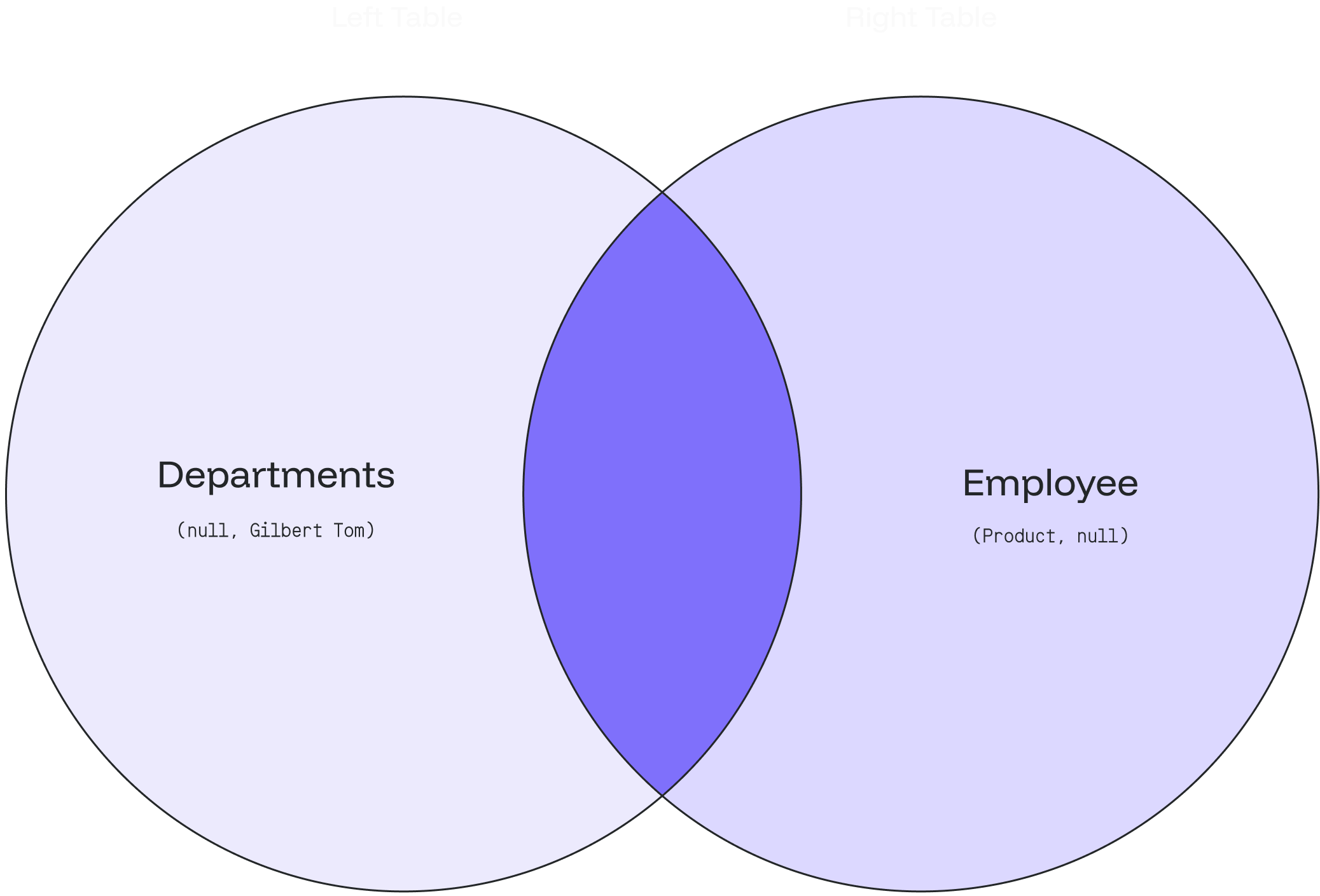
2. The result will indicate that the **Product** department doesn’t have any employees 👨🏻‍💼 ```sql theme={null} +------------------+--------------------+ | employee_name | department_name | +------------------+--------------------+ | null | Product | +------------------+--------------------+ ``` **b) Department** 1\) Let’s find out the employee who doesn’t belong to any department by adding a WHERE clause and NULL as the following query: ```sql theme={null} SELECT employee_name, department_name FROM employee FULL OUTER JOIN departments ON employee.dept_id = departments.department_id WHERE department_name IS NULL; ``` 
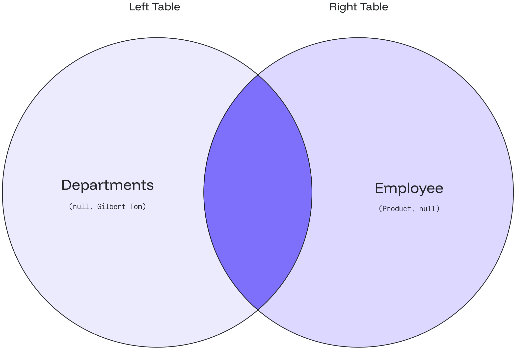
2\) The result will show that **Gilbert Tom** doesn’t belong to any department 👨🏻‍💼 ```sql theme={null} +------------------+--------------------+ | employee_name | department_name | +------------------+--------------------+ | Gilbert Tom | null | +------------------+--------------------+ ``` The following Venn diagram illustrates how the FULL OUTER JOIN works for the department and employee with a null value: --- # Source: https://docs.oxla.com/sql-reference/sql-clauses/over-window.md > ## Documentation Index > Fetch the complete documentation index at: https://docs.oxla.com/llms.txt > Use this file to discover all available pages before exploring further. # OVER / WINDOW ## Overview All window functions utilise a set of clauses specific for them, some of which are mandatory while others are optional. ## OVER Clause When it comes to required ones, there is the `OVER` clause, which defines a window or user-specified set of rows within a query result set. It is a mandatory element of window functions, defining the window specification and differentiating them from other SQL functions. ### Syntax The syntax for this clause looks as follows: ```sql theme={null} OVER (PARTITION BY rows1 ORDER BY rows2) ``` where, the `PARTITION BY` clause is a list of `expressions` interpreted in much the same fashion as the elements of a `GROUP BY` clause, with major exception that they are always simple expressions and never the name or number of an output column. Another difference is that these expressions can contain aggregate function calls, which are not allowed in a regular `GROUP BY` clause (they are allowed here because windowing occurs after grouping and aggregation) `[ PARTITION BY expression [, ...] ]` (optional window partition) The `ORDER BY` clause used in the `OVER` clause above is a list of `expressions` interpreted in much the same fashion as the elements of a statement-level `ORDER BY` clause, except that the expressions are always taken as simple expressions and never the name or number of an output column. `[ ORDER BY expression [ ASC | DESC | USING operator ] [ NULLS { FIRST | LAST } ] [, ...] ]` (optional window ordering) ## WINDOW Clause In terms of window functions' optional clauses, there is the `WINDOW` clause that defines one or more named window specification, as a `window_name` and `window_definition` pair. ### Syntax The syntax for this clause looks as follows: ```sql theme={null} WINDOW window_name AS (window_definition) [, ...] ``` where `window_name` is a name that can be referenced from the `OVER` clauses or subsequent `window definition`. There are a few important things to keep in mind here: * The `window_definition` may use an `existing_window_name` to refer to a previous `window_definition` in the `WINDOW` clause, but the previous `window_definition` must not specify a `frame` clause * The `window_definition` copies the `PARTITION BY` clause and `ORDER BY` clause from previous `window_definition`, but it cannot specify its own `PARTION BY` clause, and can specify an `ORDER BY` clause if the previous `window_definition` does not have one. `[ existing_window_name ] [ PARTITION BY clause ] [ ORDER BY clause ] [ frame clause ]` (all arguments are optional) The `window_definition` without arguments defines a window with all rows without partition and ordering The `frame` clause referenced above defines the window frame for window functions that depend on the frame (not all do). The window frame is a set of related rows for each row of the query (called the current row). * `{ RANGE | ROWS | GROUPS } frame_start [ frame_exclusion ]` * `{ RANGE | ROWS | GROUPS } BETWEEN frame_start AND frame_end [ frame_exclusion ]` The `frame` clause of the window specification is limited to the `ROWS` clause without `frame exclusion` one There are a couple of things, to keep in mind here: * `frame_start` and `frame_end` can be one of: `UNBOUNDED PRECEDING`, `offset PRECEDING`, `CURRENT ROW`, `offset FOLLOWING`, `UNBOUNDED FOLLOWING`. * If `frame_end` is omitted it defaults to `CURRENT ROW`. Restrictions here are as follows: * `frame_start` cannot be `UNBOUNDED FOLLOWING` * `frame_end` cannot be `UNBOUNDED PRECEDING` * `frame_end` choice cannot appear earlier in the above list of `frame_start` and `frame_end` options than the `frame_start` choice does In `ROWS` mode, `CURRENT ROW` means that the frame starts or ends with the current row, the offset is an integer indicating that the frame starts or ends that many rows before or after the current row. Beware that the `ROWS` mode can produce unpredictable results if the `ORDER BY` ordering does not order the rows uniquely ## Examples For the needs of this section, we will create the `winsales` table that stores details about some sales transactions: ```sql theme={null} CREATE TABLE winsales( salesid int, dateid date, sellerid int, buyerid text, qty int, qty_shipped int); INSERT INTO winsales VALUES (30001, '8/2/2003', 3, 'b', 10, 10), (10001, '12/24/2003', 1, 'c', 10, 10), (10005, '12/24/2003', 1, 'a', 30, null), (40001, '1/9/2004', 4, 'a', 40, null), (10006, '1/18/2004', 1, 'c', 10, null), (20001, '2/12/2004', 2, 'b', 20, 20), (40005, '2/12/2004', 4, 'a', 10, 10), (20002, '2/16/2004', 2, 'c', 20, 20), (30003, '4/18/2004', 3, 'b', 15, null), (30004, '4/18/2004', 3, 'b', 20, null), (30007, '9/7/2004', 3, 'c', 30, null); ``` ### OVER Clause in Window Functions with Window Definition, PARTITION BY and ORDER BY clauses In this example, we will focus on executing a window function with the `OVER` clause, window definition and `PARTITION BY` and `ORDER BY` clauses: ```sql theme={null} SELECT * SUM(qty) OVER (PARTITION BY sellerid) AS seller_qty FROM winsales ORDER BY sellerid, salesid; ``` Here's the output for the above code: ```sql theme={null} salesid | dateid | sellerid | buyerid | qty | qty_shipped | seller_qty ---------+------------+----------+---------+-----+-------------+------------ 10001 | 2003-12-24 | 1 | c | 10 | 10 | 50 10005 | 2003-12-24 | 1 | a | 30 | | 50 10006 | 2004-01-18 | 1 | c | 10 | | 50 20001 | 2004-02-12 | 2 | b | 20 | 20 | 40 20002 | 2004-02-16 | 2 | c | 20 | 20 | 40 30001 | 2003-08-02 | 3 | b | 10 | 10 | 75 30003 | 2004-04-18 | 3 | b | 15 | | 75 30004 | 2004-04-18 | 3 | b | 20 | | 75 30007 | 2004-09-07 | 3 | c | 30 | | 75 40001 | 2004-01-09 | 4 | a | 40 | | 50 40005 | 2004-02-12 | 4 | a | 10 | 10 | 50 (11 rows) ``` ### OVER Clause in Window Functions with Window Name, PARTITION BY and ORDER BY clauses In this example, we will focus on executing a window function with the `OVER` clause, window name and `PARITION BY` and `ORDER BY` clauses: ```sql theme={null} SELECT * SUM(qty) OVER seller AS seller_qty FROM winsales WINDOW seller AS (PARTITION BY sellerid) ORDER BY sellerid, salesid; ``` When executing the code above, we will get the following output: ```sql theme={null} salesid | dateid | sellerid | buyerid | qty | qty_shipped | seller_qty ---------+------------+----------+---------+-----+-------------+------------ 10001 | 2003-12-24 | 1 | c | 10 | 10 | 50 10005 | 2003-12-24 | 1 | a | 30 | | 50 10006 | 2004-01-18 | 1 | c | 10 | | 50 20001 | 2004-02-12 | 2 | b | 20 | 20 | 40 20002 | 2004-02-16 | 2 | c | 20 | 20 | 40 30001 | 2003-08-02 | 3 | b | 10 | 10 | 75 30003 | 2004-04-18 | 3 | b | 15 | | 75 30004 | 2004-04-18 | 3 | b | 20 | | 75 30007 | 2004-09-07 | 3 | c | 30 | | 75 40001 | 2004-01-09 | 4 | a | 40 | | 50 40005 | 2004-02-12 | 4 | a | 10 | 10 | 50 (11 rows) ``` --- # Source: https://docs.oxla.com/sql-reference/sql-functions/aggregate-functions/overview-statistics.md > ## Documentation Index > Fetch the complete documentation index at: https://docs.oxla.com/llms.txt > Use this file to discover all available pages before exploring further. # Overview Aggregate functions for statistics are typically used for statistical analysis. Oxla supports the following functions: | **Functions** | **Description** | | ---------------------------------------------------------------------------------- | -------------------------------------------------------------------------------------------------------------------- | | [CORR](/sql-reference/sql-functions/aggregate-functions/corr) | Calculates the Pearson correlation coefficient between two sets of number pairs | | [COVAR\_POP](/sql-reference/sql-functions/aggregate-functions/covar-pop) | Calculates the population covariance between two sets of number pairs | | [COVAR\_SAMP](/sql-reference/sql-functions/aggregate-functions/covar-samp) | Calculates the sample covariance between two sets of number pairs | | [REGR\_AVGX](/sql-reference/sql-functions/aggregate-functions/regr-avgx) | Calculates the average of the independent variable (sum(X)/N) | | [REGR\_AVGY](/sql-reference/sql-functions/aggregate-functions/regr-avgy) | Calculates the average of the dependent variable (sum(Y)/N) | | [REGR\_COUNT](/sql-reference/sql-functions/aggregate-functions/regr-count) | Calculates the number of input rows in which both expressions are non-null | | [REGR\_INTERCEPT](/sql-reference/sql-functions/aggregate-functions/regr-intercept) | Calculates the y-intercept of the univariate linear regression line for a group of data points | | [REGR\_R2](/sql-reference/sql-functions/aggregate-functions/regr-r2) | Calculates the coefficient of determination (R2) for a linear regression model | | [REGR\_SLOPE](/sql-reference/sql-functions/aggregate-functions/regr-slope) | Calculates slope of the least-squares-fit linear equation determined by the (X, Y) pairs | | [REGR\_SXX](/sql-reference/sql-functions/aggregate-functions/regr-sxx) | Calculates the sum(X2) - sum(X)2/N ("sum of squares" of the independent variable) | | [REGR\_SXY](/sql-reference/sql-functions/aggregate-functions/regr-sxy) | Calculates the sum(X\*Y) - sum(X) \* sum(Y)/N ("sum of products" of independent times dependent variable) | | [REGR\_SYY](/sql-reference/sql-functions/aggregate-functions/regr-syy) | Calculates the sum(Y2) - sum(Y)2/N ("sum of squares" of the dependent variable) | | [STDDEV](/sql-reference/sql-functions/aggregate-functions/stddev) | Calculates the sample standard deviation of a set of numeric values | | [STDDEV\_POP](/sql-reference/sql-functions/aggregate-functions/stddev-pop) | Calculates the population standard deviation of the input values | | [STDDEV\_SAMP](/sql-reference/sql-functions/aggregate-functions/stddev-samp) | Calculates the sample standard deviation of the input values | | [VARIANCE](/sql-reference/sql-functions/aggregate-functions/variance) | Calculates the the sample variance of a set of numeric values. | | [VAR\_POP](/sql-reference/sql-functions/aggregate-functions/var-pop) | Calculates the population variance of the input values (square of the population standard deviation) | | [VAR\_SAMP](/sql-reference/sql-functions/aggregate-functions/var-samp) | Calculates the sample variance of the input values (square of the sample standard deviation) | --- # Source: https://docs.oxla.com/system-catalogs/overview.md # Source: https://docs.oxla.com/sql-reference/sql-statements/overview.md # Source: https://docs.oxla.com/sql-reference/sql-mutations/overview.md # Source: https://docs.oxla.com/sql-reference/sql-functions/window-functions/overview.md # Source: https://docs.oxla.com/sql-reference/sql-functions/trigonometric-functions/overview.md # Source: https://docs.oxla.com/sql-reference/sql-functions/timestamp-functions/overview.md # Source: https://docs.oxla.com/sql-reference/sql-functions/string-functions/overview.md # Source: https://docs.oxla.com/sql-reference/sql-functions/overview.md # Source: https://docs.oxla.com/sql-reference/sql-functions/other-functions/overview.md # Source: https://docs.oxla.com/sql-reference/sql-functions/math-functions/overview.md # Source: https://docs.oxla.com/sql-reference/sql-functions/json-functions/overview.md # Source: https://docs.oxla.com/sql-reference/sql-functions/aggregate-functions/overview.md # Source: https://docs.oxla.com/sql-reference/sql-data-types/overview.md # Source: https://docs.oxla.com/sql-reference/sql-clauses/set-operations/overview.md # Source: https://docs.oxla.com/sql-reference/sql-clauses/overview.md # Source: https://docs.oxla.com/sql-reference/overview.md > ## Documentation Index > Fetch the complete documentation index at: https://docs.oxla.com/llms.txt > Use this file to discover all available pages before exploring further. # SQL Reference This section provides information about the syntax and semantics of SQL queries, clauses, data types, and functions that Oxla supports. The information in this section is divided into groups according to the kind of operation they perform as follows: } href="/sql-reference/sql-statements/overview" > Learn how to create a request for data or information from one or more database tables using our supported statements. } href="/sql-reference/sql-clauses/overview" > This sub-section show you how to write user-friendly queries and analyze data using different constraints and conditions. } href="/sql-reference/sql-data-types/overview" > This sub-section will guide you through implementing our supported data types to run your operations, such as text, timestamp, numeric, and many more… } href="/sql-reference/sql-functions/overview" > See how you can combine the statements, data types, and other references into specific functions for particular tasks. } href="/sql-reference/schema" > Learn about a logical container that holds database objects and relationships of data in a database. } href="/sql-reference/comment-support" > Adding comments in your queries for better documentation and collaboration. } href="/sql-reference/transactions" > Learn more about managing your transactions. } href="/sql-reference/sql-mutations/overview" > Modify your existing data with data manipulation. --- # Source: https://docs.oxla.com/security/ownership.md > ## Documentation Index > Fetch the complete documentation index at: https://docs.oxla.com/llms.txt > Use this file to discover all available pages before exploring further. # Ownership ## Overview In Oxla, ownership defines the relationship where objects such as databases, tables and schemas belong to a specific role. Keep the following principles in mind regarding ownership: * Indexes do not have explicit owners; the owner of the table also owns its indexes * Ownership is required to `DROP` an object * For grants validation, the owner implicitly has all privileges on the resource: * For table: `SELECT`, `INSERT`, `UPDATE`, `DELETE` * For schema: `USAGE`, `CREATE` This section explains how to check and change ownership and clarifies the differences between ownership and role privileges. ## Checking Ownership To check ownerships in Oxla, a superuser can execute the following query: ```sql theme={null} SELECT * FROM oxla_internal.oxla_object_owner; ``` Example output: ```text theme={null} id | database | schema | object_name | object_type ----+----------+--------+-----------------+------------- 5 | oxla | public | data_types_demo | TABLE ``` Here's the breakdown of the above output: * `id`: role ID * `database`: database name * `schema`: schema name (empty if `object_type` is DATABASE) * `object_name`: object name (empty if `object_type` is SCHEMA or DATABASE) * `object_type`: type of the object ## Changing Ownership To change ownership, use the following syntax: ```sql theme={null} ALTER [ TABLE | SCHEMA | DATABASE ] OBJECT_NAME OWNER TO ROLE_NAME; ``` where: * `OBJECT_NAME`: name of the object, whose ownership they want to change * `ROLE_NAME`: name of the role that will become the new owner of the specified object, or keyword CURRENT\_ROLE/CURRENT\_USER ## Ownership vs Role Privileges Unlike PostgreSQL, Oxla treats ownership and grants as independent. While owners implicitly have all privileges on their resources, these privileges: * Are not visible in `oxla_internal.oxla_role_ns_grants` or `oxla_internal.oxla_role_table_grants` * Cannot be revoked `GRANT` or `REVOKE` operations can still be performed on object owner - they will result in creating or removing entries in `oxla_internal.oxla_role_..._grants` tables, which are independent of data stored in `oxla_internal.oxla_object_owner`. These grants do not matter anything as long as the user is the owner of a given resource, but they will take effect when the owner is changed. ## Examples Here are a few examples that demonstrate the behaviours described above, assuming there is a `table1` and `user1` role with `USAGE` grant in public schema: * After the following operations `user1` will no longer be the owner of `table1`, but will have `SELECT` grant on that table. ```sql theme={null} ALTER TABLE table1 OWNER TO user1; GRANT SELECT ON table1 TO user1; ALTER TABLE table1 OWNER TO oxla; ``` * After the following operations `user1` will still be able to `SELECT` from `table1` because of ownership, however `REVOKE` does not change anything. ```sql theme={null} ALTER TABLE table1 OWNER TO user1; REVOKE SELECT ON table1 FROM user1; ``` * After the following operations `user1` will not have access to `table1`, however the owner has been changed and grant has been revoked. ```sql theme={null} ALTER TABLE table1 OWNER TO user1; GRANT SELECT ON table1 TO user1; REVOKE SELECT ON table1 FROM user1; ALTER TABLE table1 OWNER TO oxla; ``` --- # Source: https://docs.oxla.com/resources/oxla-vs-postgresql.md > ## Documentation Index > Fetch the complete documentation index at: https://docs.oxla.com/llms.txt > Use this file to discover all available pages before exploring further. # Oxla vs. PostgreSQL ## Functions ### Mathematical A mathematical function operates on input values provided as arguments and returns a numeric value as the operation's output. | **Mathematical** | **Description** | **Example** | **Available in Oxla** | | ---------------- | -------------------------------------------------------------------------------------------------------- | --------------------- | --------------------- | | ABS | Returns the absolute value of a number. | `SELECT ABS(-11);` | Available | | CEIL | Returns the value after rounding up any positive or negative value to the nearest largest integer. | `SELECT CEIL(53.7);` | Available | | FLOOR | Returns the value after rounding up any positive or negative decimal value as smaller than the argument. | `SELECT FLOOR(53.6);` | Available | | LN | Returns the natural logarithm of a given number. | `SELECT LN(3);` | Available | | RANDOM | Returns the random value between 0 and 1. | `SELECT RANDOM();` | Available | | SQRT | Returns the square root of a given positive number. | `SELECT SQRT(225);` | Available | ### Trigonometric | **Trigonometric** | **Description** | **Example** | **Available in Oxla** | | ----------------- | ----------------------------------------- | ------------------ | --------------------- | | SIN | Returns the sine of the specified radian. | `SELECT sin(0.2);` | Available | ## Operators ### Mathematical Operators Below is a list of mathematical operators available in PostgreSQL: | **Operator** | **Description** | **Example** | **Result** | **Available in Oxla** | | ------------ | --------------- | ----------------- | ---------- | --------------------- | | `+` | Addition | `SELECT 5 + 8;` | `13` | Available | | `-` | Subtraction | `SELECT 2 - 3;` | `\-1` | Available | | `-` | Negation | `SELECT -4;` | `\-4` | Available | | | | `SELECT -(-4);` | `4` | Available | | | | `SELECT 5+(-2);` | `3` | Available | | | | `SELECT 5-(-2);` | `7` | Available | | `*` | Multiplication | `SELECT 3 * 3;` | `9` | Available | | `/` | Division | `SELECT 10 / 2;` | `5` | Available | | `%` | Modulo | `SELECT 20 % 3;` | `2` | Available | | `&` | Bitwise AND | `SELECT 91 & 15;` | `11` | Available | | `#` | Bitwise XOR | `SELECT 17 # 5;` | `20` | Available | ### JSON Operators Oxla supports operators for handling JSON data. One such operator is: #### Equal Operator (`=`) This operator checks if two JSON values are identical. In Oxla, this operator is order-sensitive which means that for two JSON objects to be considered equal, their key-value pairs must appear in the exact same order. ```sql theme={null} SELECT '{"a":1, "b":"c"}'::json = '{"b":"c", "a":1}'::json; ``` **Result** ```sql theme={null} ?column? ---------- f (1 row) ``` In PostgreSQL, this operator is not order-sensitive, so the order of key-value pairs does not affect the comparison result. ## Behaviors Difference ### Output Header Missing function name in output header, PostgreSQL shows the function name, like in this example: ```sql theme={null} SELECT COS(0),LN(1); ``` ```sql theme={null} cos | ln -----+----- 1 | 0 ``` Oxla does not show the function name, like in this example: ```sql theme={null} SELECT COS(0),LN(1); ``` ```sql theme={null} f | f_1 ---+----- 1 | 0 ``` ### ABS Output Differences are also found in the ABS function, where there are differences in decimal results. The example below will return the absolute value of -1.0 ```sql theme={null} SELECT ABS(-1.0); ``` It returns 1 in Oxla, while in PostgreSQL, it produces 1.0 ## Errors Difference | **Functions** | **Input** | **Output - Oxla** | **Output - PostgreSQL** | | ------------- | --------------------- | ----------------------- | --------------------------------------------------------- | | LN | `LN(0)` | *Infinity* | *ERROR: cannot take the logarithm of zero* | | | `LN(0.0)` | *Infinity* | *ERROR: cannot take the logarithm of zero* | | LOG10 | `LOG10(-1)` | *NaN* | *ERROR: cannot take logarithm of a negative number* | | SQRT | `SQRT(-1)` | *input is out of range* | *ERROR: cannot take the square root of a negative number* | | SIN | `SELECT sin(pi()/2);` | *unknown function pi* | working as expected | --- # Source: https://docs.oxla.com/system-catalogs/oxla_home_files.md > ## Documentation Index > Fetch the complete documentation index at: https://docs.oxla.com/llms.txt > Use this file to discover all available pages before exploring further. # Oxla Home Files ## Overview The `oxla_home_files` virtual table lists all files associated with a specific table in the oxla home directory. This approach offers a more reliable way to retrieve data than simply scanning files directly. ## Fields | Field | Content | Type | | -------------- | ------------------------------------------------------------------- | ------------- | | `path` | Path relative from the oxla working directory | TEXT | | `byte_size` | Size of the file in bytes | BIGINT | | `start_index` | First index in the file, binary data base64 encoded (if applicable) | NULLABLE TEXT | | `end_index` | Last index in the file, binary data base64 encoded (if applicable) | NULLABLE TEXT | | `row_count` | Number of rows in the file | BIGINT | | `batch_count` | Number of batches the file is divided into | BIGINT | | `table_id` | ID of the related table | BIGINT | | `namespace_id` | ID of the related namespace | BIGINT | | `database_id` | ID of the related database | BIGINT | ## Example Query This example shows how to query the `oxla_home_files` table in an Oxla instance ### Empty Result 1. Run the `oxla_home_files` query below: ```sql theme={null} SELECT * FROM oxla_internal.oxla_home_files; ``` 2. When the `oxla_home_files` table is empty, the query returns an empty result set: ```sql theme={null} path | byte_size | start_index | end_index | row_count | batch_count | table_id | namespace_id | database_id ------+-----------+-------------+-----------+-----------+-------------+----------+--------------+------------- (0 rows) ``` ### After Data Insertion 1. Create and insert data into the table: ```sql theme={null} CREATE TABLE orders ( order_id INT, order_date DATE, total_amount INT, shipping_address TEXT, status TEXT ); INSERT INTO orders (order_id, order_date, total_amount, shipping_address, status) VALUES (1001, '2024-07-13', 150.75, '123 Main St, Anytown, USA', 'Shipped'), (1002, '2024-07-12', 200.50, '456 Elm St, Othertown, USA', 'Delivered'), (1003, '2024-07-12', 350.25, '789 Oak St, Anotherplace, USA', 'Processing'), (1001, '2024-07-11', 100.00, '321 Pine St, Somewhere, USA', 'Cancelled'), (1004, '2024-07-10', 500.00, '555 Maple St, Nowhere, USA', 'Pending'); ``` 2. Run the `oxla_home_files` query: ```sql theme={null} SELECT * FROM oxla_internal.oxla_home_files; ``` 3. After inserting data into the table, the query lists the file metadata stored in Oxla: ```sql theme={null} path | byte_size | start_index | end_index | row_count | batch_count | table_id | namespace_id | database_id ------------------------------------------------------------------------------------------------------------------------------------------------------------------------- /0/0/16385/buffers/cluster-2jyd1jzvhgequov20igkxe4peyl-oxla-0/0 | 978 | | | 5 | 1 | 16385 | 0 | 0 (1 row) ``` --- # Source: https://docs.oxla.com/sql-reference/sql-functions/window-functions/percent-rank.md > ## Documentation Index > Fetch the complete documentation index at: https://docs.oxla.com/llms.txt > Use this file to discover all available pages before exploring further. # PERCENT_RANK() ## Overview `PERCENT_RANK()` window function determines the relative rank of a value in a group of values, based on the `ORDER BY` expression in the `OVER` clause. It can be used with all [data types supported by Oxla](/sql-reference/sql-data-types/overview). ## Syntax The syntax for this function is as follows: ```sql theme={null} PERCENT_RANK() OVER ( [PARTITION BY partition_expression] ORDER BY sort_expression ) ``` The `PERCENT_RANK()` is calculated as: ```bash theme={null} (r - 1) / (n - 1) ``` Where `r` is the rank of the current row and `n` is the total number of rows in the window or partition. Rows with equal values for the ranking criteria receive the same relative rank. The output data type for this function is `DOUBLE PRECISION`. The output will indicate the rank of values in a table, regardless of the input types. * If the optional `PARTITION BY` expression is present, the rankings are reset for each group of rows * If the `ORDER BY` expression is omitted then all relative ranks are equal to 0 ## Parameters * `()`: this function takes no arguments but parentheses is required * `PARTITION BY`: optional clause used to divide the result set into partitions (`PERCENT_RANK()` function is applied to each partition independently) * `ORDER BY`: order of rows in each partition to which the function is applied ## Examples For the needs of this section, we will create the `winsales` table that stores details about some sales transactions: ```sql theme={null} CREATE TABLE winsales( salesid int, dateid date, sellerid int, buyerid text, qty int, qty_shipped int); INSERT INTO winsales VALUES (30001, '8/2/2003', 3, 'b', 10, 10), (10001, '12/24/2003', 1, 'c', 10, 10), (10005, '12/24/2003', 1, 'a', 30, null), (40001, '1/9/2004', 4, 'a', 40, null), (10006, '1/18/2004', 1, 'c', 10, null), (20001, '2/12/2004', 2, 'b', 20, 20), (40005, '2/12/2004', 4, 'a', 10, 10), (20002, '2/16/2004', 2, 'c', 20, 20), (30003, '4/18/2004', 3, 'b', 15, null), (30004, '4/18/2004', 3, 'b', 20, null), (30007, '9/7/2004', 3, 'c', 30, null); ``` ### PERCENT\_RANK() with ORDER BY In this example, we will focus on executing the `PERCENT_RANK()` function with `ORDER BY` keyword and calculate the descending percent rank of all rows based on the quantity sold: ```sql theme={null} SELECT salesid, qty PERCENT_RANK() OVER (ORDER BY qty DESC) AS p_rnk RANK() OVER (ORDER BY qty DESC) AS rnk FROM winsales ORDER BY 2,1; ``` Here is the output for the query presented above that includes the sales ID along with the quantity sold and both percent and regular ranks: ```sql theme={null} salesid | qty | p_rnk | rnk ---------+-----+-------+----- 10001 | 10 | 0.7 | 8 10006 | 10 | 0.7 | 8 30001 | 10 | 0.7 | 8 40005 | 10 | 0.7 | 8 30003 | 15 | 0.6 | 7 20001 | 20 | 0.3 | 4 20002 | 20 | 0.3 | 4 30004 | 20 | 0.3 | 4 10005 | 30 | 0.1 | 2 30007 | 30 | 0.1 | 2 40001 | 40 | 0 | 1 ``` ### PERCENT\_RANK() with ORDER BY and PARTITION BY In this example, we will focus on executing the `PERCENT_RANK()` function with `ORDER BY` keyword and `PARTITION BY` clause, partition the table by seller ID, order each partition by the quantity and assign a percent rank to each row: ```sql theme={null} SELECT salesid, sellerid, qty PERCENT_RANK() OVER (PARTITION BY sellerid ORDER BY qty DESC) AS p_rnk FROM winsales ORDER BY 2,3,1; ``` Here is the output for the query presented above: ```sql theme={null} salesid | sellerid | qty | p_rnk ---------+----------+-----+-------------------- 10001 | 1 | 10 | 0.5 10006 | 1 | 10 | 0.5 10005 | 1 | 30 | 0 20001 | 2 | 20 | 0 20002 | 2 | 20 | 0 30001 | 3 | 10 | 1 30003 | 3 | 15 | 0.6666666666666666 30004 | 3 | 20 | 0.3333333333333333 30007 | 3 | 30 | 0 40005 | 4 | 10 | 1 40001 | 4 | 40 | 0 (11 rows) ``` --- # Source: https://docs.oxla.com/sql-reference/sql-functions/aggregate-functions/ordered-set-aggregate-functions/percentile-cont.md > ## Documentation Index > Fetch the complete documentation index at: https://docs.oxla.com/llms.txt > Use this file to discover all available pages before exploring further. # PERCENTILE_CONT() ## Overview `PERCENTILE_CONT()` is an ordered-set aggregate function used to compute continuous percentiles from a set of values. The **continuous percentile** returns an interpolated value based on the distribution of the input data, while **multiple continuous percentiles** return an array of results matching the shape of the `fractions` parameter with each non-null element replaced by the value corresponding to that percentile.

Syntax

The syntax for this function is as follows:

handleTabChange('tab1')}>
```sql theme={null} PERCENTILE_CONT(fraction) WITHIN GROUP (ORDER BY order_list) ``` This function is often used in conjunction with the `WITHIN GROUP` clause to specify how to order the data before calculating the percentile.

Parameters

- `fraction`: decimal value between 0 and 1 representing the desired percentile (e.g. 0.25 for the 25th percentile)

handleTabChange('tab2')}>
```sql theme={null} PERCENTILE_CONT(fractions) WITHIN GROUP (ORDER BY order_list) ``` This function is often used in conjunction with the `WITHIN GROUP` clause to specify how to order the data before calculating the percentile.

Parameters

- `fractions`: array of decimal values between 0 and 1 representing the desired percentiles (e.g. `ARRAY[0.25, 0.50, 0.75, 0.90]`)

## Example For the needs of this section we will use a simplified version of the `film` table from the Pagila database, that will contain only the `title`, `length` and `rating` columns. ```sql theme={null} DROP TABLE IF EXISTS film; CREATE TABLE film ( title text NOT NULL, length int, rating text ); INSERT INTO film(title, length, rating) VALUES ('ATTRACTION NEWTON', 83, 'PG-13'), ('CHRISTMAS MOONSHINE', 150, 'NC-17'), ('DANGEROUS UPTOWN', 121, 'PG'), ('KILL BROTHERHOOD', 54, 'G'), ('HALLOWEEN NUTS', 47, 'PG-13'), ('HOURS RAGE', 122, 'NC-17'), ('PIANIST OUTFIELD', 136, 'NC-17'), ('PICKUP DRIVING', 77, 'G'), ('INDEPENDENCE HOTEL', 157, 'NC-17'), ('PRIVATE DROP', 106, 'PG'), ('SAINTS BRIDE', 125, 'G'), ('FOREVER CANDIDATE', 131, 'NC-17'), ('MILLION ACE', 142, 'PG-13'), ('SLEEPY JAPANESE', 137, 'PG'), ('WRATH MILE', 176, 'NC-17'), ('YOUTH KICK', 179, 'NC-17'), ('CLOCKWORK PARADISE', 143, 'PG-13'); ``` This query calculates the median film length within each rating category. ```SQL theme={null} SELECT rating, PERCENTILE_CONT(0.50) WITHIN GROUP (ORDER BY length) AS "50th percentile" FROM film GROUP BY rating; ``` By executing the code above we will get the following output: ```sql theme={null} rating | 25th percentile --------+----------------- PG-13 | 74 PG | 113.5 NC-17 | 133.5 G | 65.5 (4 rows) ``` --- # Source: https://docs.oxla.com/sql-reference/sql-functions/aggregate-functions/ordered-set-aggregate-functions/percentile-disc.md > ## Documentation Index > Fetch the complete documentation index at: https://docs.oxla.com/llms.txt > Use this file to discover all available pages before exploring further. # PERCENTILE_DISC() ## Overview `PERCENTILE_DISC()` is an ordered-set aggregate function used to compute discrete percentiles from a set of values. The **discrete percentile** returns the first input value, which position in the ordering equals or exceeds the specified fraction, while **multiple discrete percentiles** return an array of results matching the shape of the fractions parameter, with each non-null element being replaced by the input value corresponding to that percentile.

Syntax

The syntax for this function is as follows:

handleTabChange('tab1')}>
```sql theme={null} PERCENTILE_DISC(fraction) WITHIN GROUP (ORDER BY order_list) ``` If multiple values share the same rank at the specified percentile, `PERCENTILE_DISC()` will return the first one encountered in the ordering.

Parameters

- `fraction`: decimal value between 0 and 1 representing the desired percentile (e.g. 0.25 for the 25th percentile)

handleTabChange('tab2')}>
```sql theme={null} PERCENTILE_DISC(fractions) WITHIN GROUP (ORDER BY order_list) ``` If multiple values share the same rank at the specified percentile, `PERCENTILE_DISC` will return the first one encountered in the ordering.

Parameters

- `fractions`: array of decimal values between 0 and 1 representing the desired percentiles (e.g. `ARRAY[0.25, 0.50, 0.75, 0.90]`)

## Example For the needs of this section we will use a simplified version of the `film` table from the Pagila database, that will contain only the `title`, `length` and `rating` columns. ```sql theme={null} DROP TABLE IF EXISTS film; CREATE TABLE film ( title text NOT NULL, length int, rating text ); INSERT INTO film(title, length, rating) VALUES ('ATTRACTION NEWTON', 83, 'PG-13'), ('CHRISTMAS MOONSHINE', 150, 'NC-17'), ('DANGEROUS UPTOWN', 121, 'PG'), ('KILL BROTHERHOOD', 54, 'G'), ('HALLOWEEN NUTS', 47, 'PG-13'), ('HOURS RAGE', 122, 'NC-17'), ('PIANIST OUTFIELD', 136, 'NC-17'), ('PICKUP DRIVING', 77, 'G'), ('INDEPENDENCE HOTEL', 157, 'NC-17'), ('PRIVATE DROP', 106, 'PG'), ('SAINTS BRIDE', 125, 'G'), ('FOREVER CANDIDATE', 131, 'NC-17'), ('MILLION ACE', 142, 'PG-13'), ('SLEEPY JAPANESE', 137, 'PG'), ('WRATH MILE', 176, 'NC-17'), ('YOUTH KICK', 179, 'NC-17'), ('CLOCKWORK PARADISE', 143, 'PG-13'); ``` The query below calculates the quartile, median and the third quartile of film lengths: ```sql theme={null} SELECT rating, percentile_disc(ARRAY[0.25, 0.5, 0.75]) WITHIN GROUP (ORDER BY length) AS "quartiles" FROM film GROUP BY rating; ``` By executing the code above, we will get the following output: ```sql theme={null} rating | quartiles --------+--------------- G | {54,77,125} PG | {106,121,137} PG-13 | {47,83,142} NC-17 | {131,150,176} (4 rows) ``` --- # Source: https://docs.oxla.com/sql-reference/sql-functions/other-functions/pg-backend-pid.md > ## Documentation Index > Fetch the complete documentation index at: https://docs.oxla.com/llms.txt > Use this file to discover all available pages before exploring further. # pg_backend_pid() ## Overview The pg\_backend\_pid() is a session information function that returns the process ID (PID) of the server process handling the current session. It is useful for identifying the backend process associated with a specific database connection, allowing for monitoring and tasks management. ## Syntax The syntax for the `pg_backend_pid()` function is as follows: ```sql theme={null} pg_backend_pid() ``` --- # Source: https://docs.oxla.com/sql-reference/sql-functions/other-functions/pg-encoding-to-char.md > ## Documentation Index > Fetch the complete documentation index at: https://docs.oxla.com/llms.txt > Use this file to discover all available pages before exploring further. # pg_encoding_to_char() ## Overview The pg\_encoding\_to\_char() is a system catalog information function that converts an encoding internal identifier to a human-readable name. ## Syntax The syntax for the `pg_encoding_to_char()` function is as follows: ```sql theme={null} pg_encoding_to_char(number) ``` ## Parameters The following parameters are required to execute function: * `number`: specifies the integer value representing the encoding identifier ## Examples ```sql theme={null} SELECT pg_encoding_to_char(1); pg_encoding_to_char --------------------- EUC_JP (1 row) ``` ```sql theme={null} SELECT pg_encoding_to_char(0); pg_encoding_to_char --------------------- SQL_ASCII (1 row) ``` ```sql theme={null} SELECT pg_encoding_to_char(-1); pg_encoding_to_char --------------------- (1 row) ``` --- # Source: https://docs.oxla.com/sql-reference/sql-functions/other-functions/pg-get-constraintdef.md > ## Documentation Index > Fetch the complete documentation index at: https://docs.oxla.com/llms.txt > Use this file to discover all available pages before exploring further. # pg_get_constraintdef() ## Overview The pg\_get\_constraintdef() is a system catalog information function that retrieves the definition of a specific constraint in a human-readable format. ## Syntax The syntax for the `pg_get_constraintdef()` function is as follows:
pg\_get\_constraintdef (constraint\_oid \[, pretty\_bool]) → NULL
## Parameters The following parameters are required to execute this function: * constraint\_oid: specifies the object identifier (OID) of the constraint for which you want to retrieve the definition * pretty\_bool: controls whether to format the output in a human-readable way ## Restrictions * This function always returns `NULL` if there are no parameters specified --- # Source: https://docs.oxla.com/sql-reference/sql-functions/other-functions/pg-get-expr.md > ## Documentation Index > Fetch the complete documentation index at: https://docs.oxla.com/llms.txt > Use this file to discover all available pages before exploring further. # pg_get_expr() ## Overview The pg\_get\_expr() is a system catalog information function that retrieves the internal form of an individual expression, such as the default value for a column. ## Syntax There are two available syntax versions of the `pg_get_expr()` function: ```sql Version 1 theme={null} SELECT pg_get_expr('expr_text', relation_oid); ``` ```sql Version 2 theme={null} SELECT pg_get_expr('expr_text', relation_oid, pretty_bool); ``` Both versions of the `pg_get_expr()` function return an empty string `""`. ## Parameters The following parameters are required to execute this function: * `expr_text`: expression for which you want to obtain the internal representation (can be any string value) * `relation_oid`: OID (Object Identifier) of the table the expression belongs to (integer type) * `pretty_bool`: boolean value determining whether to format the expression in a more human-readable format (`TRUE`) or not (`FALSE`) ## Example For the needs of this section, first we will create a sample table named **employees** ```sql theme={null} CREATE TABLE employees ( id INT, name TEXT, salary TEXT ); ``` Then we will get the OID of the table ```sql theme={null} SELECT oid FROM pg_class WHERE relname = 'employees'; ``` ```sql theme={null} oid ------ 1018 ``` As the last step, we will retrieve the internal form for the `salary` column using `pg_get_expr()` function ```sql theme={null} -- Version 1 SELECT pg_get_expr('salary', 1018); -- Version 2 SELECT pg_get_expr('salary', 1018, TRUE); ``` By executing any of the queries above, we will get the following output: ```sql theme={null} pg_get_expr ------------- ``` --- # Source: https://docs.oxla.com/sql-reference/sql-functions/other-functions/pg-get-indexdef.md > ## Documentation Index > Fetch the complete documentation index at: https://docs.oxla.com/llms.txt > Use this file to discover all available pages before exploring further. # pg_get_indexdef() ## Overview The pg\_get\_indexdef() is a system catalog information function that reconstructs the PostgreSQL command used to retrieve the definition of a specified index. ## Syntax Here are the two available syntax versions of the `pg_get_indexdef()` function: ```sql Version 1 theme={null} pg_get_indexdef(index_oid, column_oid) ``` ```sql Version 2 theme={null} pg_get_indexdef(index_oid, column_oid, pretty_bool) ``` ## Parameters The following parameters are required to execute this function: * `index_oid`: specifies the object identifier (OID) of the index * `column_oid`: indicates the column number within the index (starting from 1) * `pretty_bool`: controls whether to format the output in a human-readable way ## Example In this example we'll start from creating a sample table and an index for it ```sql theme={null} CREATE TABLE sample_table(col int); CREATE INDEX sample_index ON sample_table(col); ``` Once that is done, we can get the OID of the index in a following way ```sql theme={null} SELECT oid FROM pg_class WHERE relname = 'sample_index'; ``` ```sql theme={null} oid ------ 16387 ``` As the last step we're going to retrieve the index definition ```sql theme={null} SELECT pg_get_indexdef(16387); ``` Here is the reconstructed definition: ```sql theme={null} pg_get_indexdef ------------------------------------------------------- CREATE INDEX sample_index ON public.sample_table(col) (1 row) ``` --- # Source: https://docs.oxla.com/sql-reference/sql-functions/other-functions/pg-get-statisticsobjdef-columns.md > ## Documentation Index > Fetch the complete documentation index at: https://docs.oxla.com/llms.txt > Use this file to discover all available pages before exploring further. # pg_get_statisticsobjdef_columns() ## Overview The pg\_get\_statisticsobjdef\_columns() is a system catalog information function that retrieves information about the columns associated with an extended statistics object. ## Syntax The syntax for the `pg_get_statisticsobjdef_columns()` function is as follows:
pg\_get\_statisticsobjdef\_columns() → NULL
## Restrictions * This function always returns `NULL` if there are no parameters specified --- # Source: https://docs.oxla.com/sql-reference/sql-functions/other-functions/pg-get-userbyid.md > ## Documentation Index > Fetch the complete documentation index at: https://docs.oxla.com/llms.txt > Use this file to discover all available pages before exploring further. # pg_get_userbyid() ## Overview The pg\_get\_userbyid() is a system catalog information function that retrieves that name of a user (role) given its unique identifier (OID). ## Syntax The syntax for the `pg_get_userbyid()` function is as follows: ```sql theme={null} pg_get_userbyid(role_oid) ``` ## Parameters The following parameters are required to execute this function: * `role_oid`: specifies the object identifier (OIDs) of the users ## Example In this example, what we will do first is to get the OIDs of all the users ```sql theme={null} SELECT id,name FROM oxla_internal.oxla_role; ``` Then, return the list of users with their ids (OIDs): ```sql theme={null} id | name ----+--------- 1 | oxla 2 | other_user (2 rows) ``` As the next step we will translate the OID to a role name in a following way: ```sql theme={null} SELECT pg_get_userbyid(2); ``` By executing the code above, we will get the following result: ```sql theme={null} pg_get_userbyid ----------------- other_user (1 row) ``` --- # Source: https://docs.oxla.com/sql-reference/sql-functions/other-functions/pg-relation-is-publishable.md > ## Documentation Index > Fetch the complete documentation index at: https://docs.oxla.com/llms.txt > Use this file to discover all available pages before exploring further. # pg_relation_is_publishable() ## Overview The`pg_relation_is_publishable()` function is used to determine whether a specified relation (table) can be published in a publication. ## Syntax The syntax for the `pg_relation_is_publishable()` function is as follows:
pg\_relation\_is\_publishable(table\_name\_or\_oid)
The function returns `false` for every existing table and `NULL` for any non-existing table. ## Parameters The following parameters are required to execute this function: * `table_name_or_oid`: specifies the object identifier (OID) of a table or it's name ## Examples ```sql theme={null} SELECT pg_relation_is_publishable('existing_table'); pg_relation_is_publishable ---------------------------- f ``` ```sql theme={null} SELECT pg_relation_is_publishable(16386); pg_relation_is_publishable ---------------------------- f ``` --- # Source: https://docs.oxla.com/sql-reference/sql-functions/other-functions/pg-size-pretty.md > ## Documentation Index > Fetch the complete documentation index at: https://docs.oxla.com/llms.txt > Use this file to discover all available pages before exploring further. # pg_size_pretty() ## Overview The pg\_size\_pretty() is a database object management function that converts sizes in bytes into a human-readable format. ## Syntax The syntax for the `pg_size_pretty()` function is as follows: ```sql theme={null} pg_size_pretty(size) ``` ## Parameters The following parameters are required to execute this function: * `size`: specifies the size in bytes that you want to convert ## Examples ```sql theme={null} SELECT pg_size_pretty(100); pg_size_pretty ---------------- 100 bytes (1 row) ``` ```sql theme={null} SELECT pg_size_pretty(1000000); pg_size_pretty ---------------- 977 kB (1 row) ``` --- # Source: https://docs.oxla.com/sql-reference/sql-functions/other-functions/pg-table-is-visible.md > ## Documentation Index > Fetch the complete documentation index at: https://docs.oxla.com/llms.txt > Use this file to discover all available pages before exploring further. # pg_table_is_visible() ## Overview The pg\_table\_is\_visible() is a schema visibility inquiry function that checks whether a specified table or other database object is visible in the current schema search path. ## Syntax The syntax for the `pg_table_is_visible()` function is as follows:
pg\_table\_is\_visible(table\_or\_index\_oid)
## Parameters The following parameters are required to run this function: * `table_or_index_oid`: specifies the object identifier (OID) of a table or it's name ## Examples ```sql theme={null} SELECT pg_table_is_visible(-1); pg_table_is_visible ---------------------------- ``` ```sql theme={null} SELECT pg_table_is_visible(16386); pg_table_is_visible ---------------------------- t ``` ```sql theme={null} SELECT pg_table_is_visible(16381); pg_table_is_visible ---------------------------- f ``` --- # Source: https://docs.oxla.com/sql-reference/sql-functions/other-functions/pg-table-size.md > ## Documentation Index > Fetch the complete documentation index at: https://docs.oxla.com/llms.txt > Use this file to discover all available pages before exploring further. # pg_table_size() ## Overview The pg\_table\_size() is a system administration function that retrieves the size of a specific table, including its associated storage components but excluding indexes. ## Syntax The syntax for the `pg_table_size()` function is as follows: ```sql theme={null} pg_table_size(regclass) ``` ## Parameters The following parameters are required to execute this function: * `regclass`: name or object identifier (OID) of the table whose size is to be retrieved --- # Source: https://docs.oxla.com/sql-reference/sql-functions/other-functions/pg-total-relation-size.md > ## Documentation Index > Fetch the complete documentation index at: https://docs.oxla.com/llms.txt > Use this file to discover all available pages before exploring further. # pg_total_relation_size() ## Overview The pg\_total\_relation\_size() is a database object size function that retrieves the size of a table and is useful for monitoring the storage requirements. ## Syntax The syntax for the `pg_total_relation_size()` function is as follows: ```sql theme={null} pg_total_relation_size('relation_name'); ``` It returns the size of the specified table in bytes. ## Parameters The following parameters are required to execute this function: * `relation_name`: name of the table for which you want to determine the size ## Example For the needs of this section, we will create a **users** table ```sql theme={null} CREATE TABLE users ( username TEXT, email TEXT ); INSERT INTO users (username, email) VALUES ('john_doe', 'john.doe@example.com'), ('jane_smith', 'jane.smith@example.com'), ('alice_smith', 'alice.smith@example.com'), ('bob_jones', 'bob.jones@example.com'), ('susan_wilson', 'susan.wilson@example.com'), ('michael_jackson', 'michael.jackson@example.com'), ('lisa_johnson', 'lisa.johnson@example.com'), ('david_smith', 'david.smith@example.com'); ``` Now we would like to use the `pg_total_relation_size()` function to determine the size of the **users** table (in bytes) ```sql theme={null} SELECT pg_total_relation_size('users'); ``` By executing the query above, we will get the following output: ```sql theme={null} pg_total_relation_size ------------------------ 556 ``` --- # Source: https://docs.oxla.com/sql-reference/sql-functions/other-functions/pg-typeof.md > ## Documentation Index > Fetch the complete documentation index at: https://docs.oxla.com/llms.txt > Use this file to discover all available pages before exploring further. # pg_typeof() ## Overview The pg\_typeof() is a system catalog information function that retrieves the data type of any given value. It returns a string literal corresponding to the expression type. ## Syntax The syntax of the `pg_typeof()` function is as follows: ```sql theme={null} SELECT pg_typeof(`any`); ``` ## Parameters The following parameters are required to execute this function: * `any`: represents any value you want to determine the data type of ## Examples ### Numeric This example shows the function usage with a numeric value: ```sql theme={null} SELECT pg_typeof(100) as "data type"; ``` ```sql theme={null} data type ----------- integer ``` ### String In this example, we will use a string value as an input: ```sql theme={null} SELECT pg_typeof('event'::TEXT) as "data type"; ``` ```sql theme={null} data type ----------- text ``` ### Interval Here we will focus on using an interval input: ```sql theme={null} SELECT pg_typeof(INTERVAL '1 day') as "data type"; ``` ```sql theme={null} data type ----------- interval ``` ### Table For the needs of this section we will create a sample table and then use `pg_typeof()` to retrieve the data types of information stored in the table ```sql theme={null} CREATE TABLE timestamp_example ( id int, event_time timestamp, description text ); INSERT INTO timestamp_example (event_time, description) VALUES ('2023-10-20 12:30:00', 'Event 1'), (NULL, 'Event 2'); ``` Now that we created the table, let's use `pg_typeof()` function to determine the data types of the **event\_time** and description columns for each row ```sql theme={null} SELECT pg_typeof(event_time) AS event_time_type, pg_typeof(description) AS description_type FROM timestamp_example; ``` By executing the query above we will get the following output ```sql theme={null} event_time_type | description_type -----------------------------+------------------ timestamp without time zone | text timestamp without time zone | text ``` --- # Source: https://docs.oxla.com/system-catalogs/catalogs/pg_attrdef.md > ## Documentation Index > Fetch the complete documentation index at: https://docs.oxla.com/llms.txt > Use this file to discover all available pages before exploring further. # pg_attrdef ## Overview The `pg_attrdef` stores information about column default values. It mimics the [pg\_attrdef](https://www.postgresql.org/docs/current/catalog-pg-attrdef.html) PostgreSQL system catalog. Please note that Oxla doesn’t support the custom types ## Columns This table is designed for compatibility with tools that require PostgreSQL system tables, so it mostly has dummy data. Please note that not all columns in `pg_attrdef` are applicable to every type of relation. The following columns are available for querying in `pg_attrdef`: | Column | Type | Description | | --------- | ------ | ---------------------------------------------------------------- | | `oid` | `int` | This column represents the row identifier | | `adrelid` | `int` | This column represents the table to which this column belongs | | `adnum` | `int` | This column represents the number of the column within the table | | `adbin` | `text` | This column represents the default value for the column | --- # Source: https://docs.oxla.com/system-catalogs/catalogs/pg_attribute.md > ## Documentation Index > Fetch the complete documentation index at: https://docs.oxla.com/llms.txt > Use this file to discover all available pages before exploring further. # pg_attribute ## Overview The `pg_attribute` stores information about table columns. It mimics the [pg\_attribute](https://www.postgresql.org/docs/current/catalog-pg-attribute.html) PostgreSQL system catalog. ## Columns This table is designed for compatibility with tools that require PostgreSQL system tables, so it mostly has dummy data. Please note that not all columns in `pg_attribute` are applicable to every type of relation The following columns are available for querying in `pg_attribute`: | Column | Type | Description | | ---------------- | ------ | --------------------------------------------------------------------------------------------- | | `attrelid` | `int` | This column represents the OID of the table (See `pg_class`) | | `attname` | `text` | This column represents the column name as specified in `CREATE TABLE` | | `atttypid` | `int` | This column represents the OID of the column type (See `pg_type`) | | `attnum` | `int` | This column represents the column index (1-based) | | `attlen` | `int` | This column represents the byte size of the value (-1 for varying length types) | | `attnotnull` | `bool` | This column represents the not-null constraint. `true` if the column was declared as NOT NULL | | `attcacheoff` | `int` | *Unused*. | | `atttypmod` | `int` | *Unused*. | | `attndims` | `int` | *Unused*. | | `attbyval` | `bool` | *Unused*. | | `attalign` | `text` | *Unused*. | | `attstorage` | `text` | *Unused*. | | `attcompression` | `text` | *Unused*. | | `atthasdef` | `bool` | *Unused*. | | `atthasmissing` | `bool` | *Unused*. | | `attidentity` | `text` | *Unused*. | | `attgenerated` | `text` | *Unused*. | | `attisdropped` | `bool` | *Unused*. | | `attislocal` | `bool` | *Unused*. | | `attinhcount` | `int` | *Unused*. | | `attstattarget` | `int` | *Unused*. | | `attcollation` | `int` | *Unused*. | | `attacl` | `text` | *Unused*. | | `attoptions` | `text` | *Unused*. | | `attfdwoptions` | `text` | *Unused*. | | `attmissingval` | `text` | *Unused*. | ## Example ### Retrieving Column Information for All Tables 1. This example queries the `pg_attribute` to retrieve information about all columns across all tables in the database: ```sql theme={null} SELECT attrelid, attname, atttypid, attnum FROM pg_attribute; ``` ```sql theme={null} attrelid | attname | atttypid | attnum ----------+---------------------+----------+-------- 100 | oid | 23 | 1 100 | nspname | 25 | 2 100 | nspowner | 23 | 3 100 | nspacl | 25 | 4 101 | indexrelid | 23 | 1 101 | indrelid | 23 | 2 101 | indnatts | 23 | 3 101 | indnkeyatts | 23 | 4 101 | indisunique | 16 | 5 101 | indnullsnotdistinct | 16 | 6 101 | indisprimary | 16 | 7 101 | indisexclusion | 16 | 8 101 | indimmediate | 16 | 9 101 | indisclustered | 16 | 10 101 | indisvalid | 16 | 11 101 | indcheckxmin | 16 | 12 101 | indisready | 16 | 13 101 | indislive | 16 | 14 101 | indisreplident | 16 | 15 101 | indkey | 23 | 16 101 | indcollation | 23 | 17 101 | indclass | 23 | 18 101 | indoption | 23 | 19 101 | indexprs | 23 | 20 101 | indpred | 23 | 21 (25 rows) ``` If your database has many tables, the result could be quite long. You can manage the output by filtering specific criteria using `WHERE` clauses or by limiting the number of rows with `LIMIT` clauses ### Filtering Columns 1. Create a new table: ```sql theme={null} CREATE TABLE books ( book_id int, title text, author text, genre text, publication_year int ); ``` 2. To get the OID (Object Identifier) of the **books** table, run the `pg_class.oid` query: ```sql theme={null} SELECT oid, relname FROM pg_class WHERE relname = 'books'; ``` 3. It will return the **books** table with its OID: ```sql theme={null} oid | relname ------+--------- 1009 | books ``` 4. To filter columns, we need to utilize the `pg_attribute` with `WHERE` clause: ```sql theme={null} SELECT attrelid, attname, atttypid, attnum FROM pg_attribute WHERE attrelid = 1009; ``` 5. The output should provide you with columns of the **books** table that you’ve just created: ```sql theme={null} attrelid | attname | atttypid | attnum ----------+------------------+----------+-------- 1009 | book_id | 23 | 1 1009 | title | 25 | 2 1009 | author | 25 | 3 1009 | genre | 25 | 4 1009 | publication_year | 23 | 5 ``` ### Joining pg\_attribute with pg\_class for Table and Column Names 1. In this example, a join operation with `pg_class` is performed to include the name of the table (`relname`): ```sql theme={null} SELECT attrelid, relname, attname, atttypid, attnum FROM pg_attribute JOIN pg_class ON attrelid = oid; ``` 2. You will receive both table and column details in a single query result: ```sql theme={null} attrelid | relname | attname | atttypid | attnum ----------+------------------+---------------+----------+-------- 1000 | client | client_id | 23 | 1 1000 | client | client_name | 25 | 2 1000 | client | client_origin | 25 | 3 1001 | distance_table | distance | 23 | 1 1001 | distance_table | unit | 25 | 2 1002 | weight | kilo | 23 | 1 1002 | weight | gram | 23 | 2 1003 | product | id | 23 | 1 1003 | product | product | 25 | 2 1003 | product | category | 25 | 3 1003 | product | price | 23 | 4 1004 | salary | empid | 23 | 1 1004 | salary | empname | 25 | 2 1004 | salary | empdept | 25 | 3 1004 | salary | empaddress | 25 | 4 1004 | salary | empsalary | 23 | 5 1005 | customer | cust_id | 23 | 1 1005 | customer | cust_name | 25 | 2 1006 | personal_details | id | 23 | 1 1006 | personal_details | first_name | 25 | 2 1006 | personal_details | last_name | 25 | 3 1006 | personal_details | gender | 25 | 4 ``` --- # Source: https://docs.oxla.com/system-catalogs/catalogs/pg_class.md > ## Documentation Index > Fetch the complete documentation index at: https://docs.oxla.com/llms.txt > Use this file to discover all available pages before exploring further. # pg_class ## Overview The `pg_class` stores information about tables and indexes in the database. It contains exactly one row per table (or index) created in the database. It mimics the [pg\_class](https://www.postgresql.org/docs/15/catalog-pg-class.html) PostgreSQL system catalog. ## Columns This table is designed for compatibility with tools that require PostgreSQL system tables, so it mostly has dummy data. Please note that not all columns in `pg_class` are applicable to every type of relation. The following columns are available for querying in `pg_class`: | Column | Type | Description | | --------------------- | ------- | ------------------------------------------------------------------------------------ | | `oid` | `int` | This column represents the table/index object ID (OID) generated by oxla | | `relname` | `text` | This column represents the table/index name as specified by the user during creation | | `relnamespace` | `int` | This column represents the OID of the namespace the relation resides in | | `relhasindex` | `bool` | Returns `true` if the table has any indexes | | `relkind` | `text` | This column represents the type of relation: `r` for tables and `i` for indexes | | `reltype` | `int` | *Unused* | | `reloftype` | `int` | *Unused* | | `relowner` | `int` | *Unused* | | `relam` | `int` | *Unused* | | `relfilenode` | `int` | *Unused* | | `reltablespace` | `int` | *Unused* | | `relpages` | `int` | *Unused* | | `reltuples` | `float` | *Unused* | | `relallvisible` | `int` | *Unused* | | `reltoastrelid` | `int` | *Unused* | | `relisshared` | `bool` | *Unused* | | `relpersistence` | `text` | *Unused* | | `relnatts` | `int` | *Unused* | | `relchecks` | `int` | *Unused* | | `relhasrules` | `bool` | *Unused* | | `relhastriggers` | `bool` | *Unused* | | `relhassubclass` | `bool` | *Unused* | | `relrowsecurity` | `bool` | *Unused* | | `relforcerowsecurity` | `bool` | *Unused* | | `relispopulated` | `bool` | *Unused* | | `relreplident` | `text` | *Unused* | | `relispartition` | `bool` | *Unused* | | `relrewrite` | `int` | *Unused* | | `relfrozenxid` | `int` | *Unused* | | `relacl` | `text` | *Unused* | | `reloptions` | `text` | *Unused* | | `relminmxid` | `text` | *Unused* | | `relpartbound` | `text` | *Unused* | ## Example 1. Create a table and define its schema: ```sql theme={null} CREATE TABLE customer_orders ( order_id INT, customer_id INT, order_date DATE, total_amount INT ); ``` 2. Create an index on the `customer_orders` table for the `customer_id` column: ```sql theme={null} CREATE INDEX idx_customer_id ON customer_orders (customer_id); ``` 3. Query the `pg_class` catalog to retrieve information about the `customer_orders` table and the index you’ve just created: ```sql theme={null} SELECT oid, relname, relkind, relhasindex, relnamespace FROM pg_class WHERE relname IN ('customer_orders', 'idx_customer_id'); ``` 4. The query will return information about the `customer_orders` table and the index: ```sql theme={null} oid | relname | relkind | relhasindex | relnamespace ------+-----------------+---------+-------------+-------------- 1013 | idx_customer_id | i | f | 0 1012 | customer_orders | r | t | 0 (2 rows) ``` --- # Source: https://docs.oxla.com/system-catalogs/catalogs/pg_constraint.md > ## Documentation Index > Fetch the complete documentation index at: https://docs.oxla.com/llms.txt > Use this file to discover all available pages before exploring further. # pg_constraint ## Overview The `pg_constraint` stores information about table constraints. It mimics the [pg\_constraint](https://www.postgresql.org/docs/current/catalog-pg-constraint.html) PostgreSQL system catalog. Please note that Oxla doesn’t support the custom types ## Columns This table is designed for compatibility with tools that require PostgreSQL system tables, so it mostly has dummy data. Please note that not all columns in `pg_constraint` are applicable to every type of relation. The following columns are available for querying in `pg_constraint`: | Column | Type | Description | | ---------------- | ------ | ------------------------------------------------------------------ | | `oid` | `int` | This column represents the row identifier | | `conname` | `text` | This column represents the constraint name | | `connamespace` | `int` | This column represents the namespace that contains this constraint | | `contype` | `text` | **unused** | | `condeferrable` | `bool` | **unused** | | `condeferred` | `bool` | **unused** | | `convalidated` | `bool` | **unused** | | `conrelid` | `int` | **unused** | | `contypid` | `int` | **unused** | | `conindid` | `int` | **unused** | | `conparentid` | `int` | **unused** | | `confrelid` | `int` | **unused** | | `confupdtype` | `text` | **unused** | | `confdeltype` | `text` | **unused** | | `confmatchtype` | `text` | **unused** | | `conislocal` | `bool` | **unused** | | `coninhcount` | `int` | **unused** | | `connoinherit` | `bool` | **unused** | | `conkey` | `text` | **unused** | | `confkey` | `text` | **unused** | | `conpfeqop` | `text` | **unused** | | `conppeqop` | `text` | **unused** | | `conffeqop` | `text` | **unused** | | `confdelsetcols` | `text` | **unused** | | `conexclop` | `text` | **unused** | | `conbin` | `text` | **unused** | --- # Source: https://docs.oxla.com/system-catalogs/catalogs/pg_depend.md > ## Documentation Index > Fetch the complete documentation index at: https://docs.oxla.com/llms.txt > Use this file to discover all available pages before exploring further. # pg_depend ## Overview The `pg_depend` tracks relationships between database objects, such as tables, columns, constraints, and indexes. It mimics the [pg\_depend](https://www.postgresql.org/docs/current/catalog-pg-depend.html) PostgreSQL system catalog. Please note that Oxla doesn’t support the custom types ## Columns This table is designed for compatibility with tools that require PostgreSQL system tables, so it mostly has dummy data. Please note that not all columns in `pg_depend` are applicable to every type of relation. The following columns are available for querying in `pg_depend`: | Column | Type | Description | | ------------- | ------ | -------------------------------------------------------------------------------- | | `classid` | `int` | This column represents the OID of the system catalog the dependent object is in | | `objid` | `int` | This column represents the OID of the specific dependent object | | `objsubid` | `int` | This column represents the column number for a table column | | `refclassid` | `int` | This column represents the OID of the system catalog the referenced object is in | | `refobjid` | `int` | This column represents the OID of the specific referenced object | | `refobjsubid` | `int` | This column represents the column number for a table column | | `deptype` | `text` | **unused** | --- # Source: https://docs.oxla.com/system-catalogs/catalogs/pg_description.md > ## Documentation Index > Fetch the complete documentation index at: https://docs.oxla.com/llms.txt > Use this file to discover all available pages before exploring further. # pg_description ## Overview The `pg_description` stores descriptions (comments) for each database object. It mimics the [pg\_description](https://www.postgresql.org/docs/current/catalog-pg-description.html) PostgreSQL system catalog. ## Columns This table is designed for compatibility with tools that require PostgreSQL system tables, so it mostly has dummy data. Please note that not all columns in `pg_description` are applicable to every type of relation. The following columns are available for querying in `pg_description`: | Column | Type | Description | | ------------- | ------ | ---------------------------------------------------------------------------------------------------------------------------------------- | | `objoid` | `int` | This column represents the OID (Object ID) of the object for which the description is stored | | `classoid` | `int` | This column represents the OID of the table that the object belongs to | | `objsubid` | `int` | If an object has multiple parts (for example, columns in a table), `objsubid` specifies the column number. If not used, this is set to 0 | | `description` | `text` | This column represents the description for the specified object | --- # Source: https://docs.oxla.com/system-catalogs/catalogs/pg_index.md > ## Documentation Index > Fetch the complete documentation index at: https://docs.oxla.com/llms.txt > Use this file to discover all available pages before exploring further. # pg_index ## Overview The `pg_index` stores information about indexes on tables. It mimics the [pg\_index](https://www.postgresql.org/docs/current/catalog-pg-index.html) PostgreSQL system catalog. ## Columns This table is designed for compatibility with tools that require PostgreSQL system tables, so it mostly has dummy data. Please note that not all columns in `pg_index` are applicable to every type of relation. The following columns are available for querying in `pg_index`: | Column | Type | Description | | --------------------- | ------ | --------------------------------------------------------------------------------- | | `indexrelid` | `int` | This column represents OID of the index | | `indrelid` | `int` | This column represents OID (Object ID) of the table on which the index is defined | | `indnatts` | `int` | This column represents number of columns in the index | | `indnkeyatts` | `int` | This column represents number of key columns in the index | | `indisunique` | `bool` | The default value is `false` | | `indnullsnotdistinct` | `bool` | *unused* | | `indisprimary` | `bool` | *unused* | | `indisexclusion` | `bool` | *unused* | | `indimmediate` | `bool` | *unused* | | `indisclustered` | `bool` | *unused* | | `indisvalid` | `bool` | *unused* | | `indcheckxmin` | `bool` | *unused* | | `indisready` | `bool` | *unused* | | `indislive` | `bool` | *unused* | | `indisreplident` | `bool` | *unused* | | `indkey` | `int` | *unused* | | `indcollation` | `int` | *unused* | | `indclass` | `int` | *unused* | | `indoption` | `int` | *unused* | | `indexprs` | `int` | *unused* | | `indpred` | `int` | *unused* | --- # Source: https://docs.oxla.com/system-catalogs/catalogs/pg_namespace.md > ## Documentation Index > Fetch the complete documentation index at: https://docs.oxla.com/llms.txt > Use this file to discover all available pages before exploring further. # pg_namespace ## Overview The `pg_namespace` contains information about schema definitions. It mimics the [pg\_namespace](https://www.postgresql.org/docs/current/catalog-pg-namespace.html) PostgreSQL system catalog. To learn more about Schema and how it is managed in Oxla, please refer to the [schema documentation](/sql-reference/schema). ## Columns This table is designed for compatibility with tools that require PostgreSQL system tables, so it mostly has dummy data. Please note that not all columns in `pg_namespace` are applicable to every type of relation. The `pg_namespace` catalog has the following key columns: | Column | Type | Description | | ---------- | ------ | ------------------------------------------------------------------------------------ | | `oid` | `int` | This column represents the Object ID, a unique identifier assigned to each namespace | | `nspname` | `text` | This column represents the name of the namespace | | `nspowner` | `int` | This column represents the owner of the namespace | | `nspacl` | `text` | *unused* | ## Example ### 1. Create a Schema In this example, we create "sales" and "hr" schemas using the query below: ```sql theme={null} CREATE SCHEMA sales; CREATE SCHEMA hr; ``` The successful result would look like this: ```sql theme={null} COMPLETE COMPLETE ``` ### 2. View Schema Definitions We then use a `SELECT` statement on the `pg_namespace` catalog to show the schema definitions. ```sql theme={null} SELECT nspname AS schema_name, oid AS schema_oid FROM pg_namespace; ``` The result shows the list of schemas and its ID, as shown below: ```sql theme={null} schema_name | schema_oid -------------+------------ public | 0 sales | 3 hr | 4 ``` --- # Source: https://docs.oxla.com/system-catalogs/catalogs/pg_settings.md > ## Documentation Index > Fetch the complete documentation index at: https://docs.oxla.com/llms.txt > Use this file to discover all available pages before exploring further. # pg_settings ## Overview The `pg_settings` displays the configuration settings for the current session. It mimics the [pg\_settings](https://www.postgresql.org/docs/current/catalog-pg-db-role-setting.html) PostgreSQL system catalog. ## Columns This table is designed for compatibility with tools that require PostgreSQL system tables, so it mostly has dummy data. Please note that not all columns in `pg_settings` are applicable to every type of relation. The following columns are available for querying in `pg_settings`: | Column | Type | Description | | ----------------- | ------ | ---------------------------------------------------------------- | | `name` | `text` | This column represents the run-time configuration parameter name | | `setting` | `text` | This column represents the current value of the parameter | | `unit` | `text` | *Unused*. | | `category` | `text` | *Unused*. | | `short_desc` | `text` | *Unused*. | | `extra_desc` | `text` | *Unused*. | | `context` | `text` | *Unused*. | | `vartype` | `text` | *Unused*. | | `source` | `text` | *Unused*. | | `min_val` | `text` | *Unused*. | | `max_val` | `text` | *Unused*. | | `enumvals` | `text` | *Unused*. | | `boot_val` | `text` | *Unused*. | | `reset_val` | `text` | *Unused*. | | `sourcefile` | `text` | *Unused*. | | `sourceline` | `int` | *Unused*. | | `pending_restart` | `bool` | *Unused*. | ## Example To retrieve information from the pg\_settings catalog, you can execute a query like: ```sql theme={null} SELECT name, setting FROM pg_settings; ``` You will get the run-time configuration values as shown below. ```sql theme={null} name | setting ----------------+--------- max_index_keys | 32 ``` --- # Source: https://docs.oxla.com/system-catalogs/catalogs/pg_statio_user_tables.md > ## Documentation Index > Fetch the complete documentation index at: https://docs.oxla.com/llms.txt > Use this file to discover all available pages before exploring further. # pg_statio_user_tables ## Overview The `pg_statio_user_tables` contains one row for each user table in the current database, showing statistics columns filled with zeros. ## Columns This table is designed for compatibility with tools that require PostgreSQL system tables, so it mostly has dummy data. Please note that not all columns in `pg_statio_user_tables` are applicable to every type of relation The following columns are available for querying in `pg_statio_user_tables` : | Column | Type | Description | | ----------------- | ------ | ------------------------------------------------------------ | | `relid` | `int` | This column represents the table ID | | `relname` | `text` | This column represents the table name | | `schemaname` | `text` | This column represents the schema name that this table is in | | `heap_blks_read` | `int` | *unused* | | `heap_blks_hit` | `int` | *unused* | | `idx_blks_read` | `int` | *unused* | | `idx_blks_hit` | `int` | *unused* | | `toast_blks_read` | `int` | *unused* | | `toast_blks_hit` | `int` | *unused* | | `tidx_blks_read` | `int` | *unused* | | `tidx_blks_hit` | `int` | *unused* | ## Example 1. Create a new table: ```sql theme={null} CREATE TABLE example_table ( data text, cluster text, storage int ); ``` 2. Run the query combined with a `WHERE` clause to look up based on the table name (`relname`): ```sql theme={null} SELECT relid, schemaname, relname FROM pg_statio_user_tables; ``` 3. It will return the table size in bytes: ```sql theme={null} relid | schemaname | relname -------+------------+--------------- 16384 | public | job 16385 | public | example_table (2 rows) ``` --- # Source: https://docs.oxla.com/system-catalogs/catalogs/pg_type.md > ## Documentation Index > Fetch the complete documentation index at: https://docs.oxla.com/llms.txt > Use this file to discover all available pages before exploring further. # pg_type ## Overview The `pg_type` table stores information about built-in data types. It mimics the [pg\_type](https://www.postgresql.org/docs/current/catalog-pg-type.html) PostgreSQL system catalog. Please note that Oxla doesn’t support the custom types ## Columns This table is designed for compatibility with tools that require PostgreSQL system tables, so it mostly has dummy data. Please note that not all columns in `pg_type` are applicable to every type of relation. The following columns are available for querying in `pg_type`: | Column | Type | Description | | ---------------- | ------ | ------------------------------------------------------------------------------------- | | `oid` | `int` | This column represents the Object ID (OID) for each type in the database | | `typname` | `text` | This column represents the data type. | | `typlen` | `int` | This column represents the number of bytes in the internal representation of the type | | `typnamespace` | `int` | *Unused* | | `typowner` | `int` | *Unused* | | `typtype` | `text` | *Unused* | | `typisdefined` | `bool` | *Unused* | | `typstorage` | `text` | *Unused* | | `typalign` | `text` | *Unused* | | `typnotnull` | `bool` | *Unused* | | `typcategory` | `text` | *Unused* | | `typispreferred` | `bool` | *Unused* | | `typdelim` | `text` | *Unused* | | `typrelid` | `int` | *Unused* | | `typsubscript` | `int` | *Unused* | | `typelem` | `int` | *Unused* | | `typarray` | `int` | *Unused* | | `typinput` | `int` | *Unused* | | `typoutput` | `int` | *Unused* | | `typreceive` | `int` | *Unused* | | `typsend` | `int` | *Unused* | | `typmodin` | `int` | *Unused* | | `typmodout` | `int` | *Unused* | | `typanalyze` | `int` | *Unused* | | `typalign` | `text` | *Unused* | | `typstorage` | `text` | *Unused* | | `typnotnull` | `bool` | *Unused* | | `typbasetype` | `int` | *Unused* | | `typtypmod` | `int` | *Unused* | | `typndims` | `int` | *Unused* | | `typcollation` | `int` | *Unused* | | `typdefaultbin` | `text` | *Unused* | | `typdefault` | `text` | *Unused* | | `typacl` | `text` | *Unused* | ## Example This example query retrieves the Object ID (`oid`) and data type name (`typname`) from the `pg_type` catalog. You can adjust the columns in the `SELECT` statement based on your needs. ```sql theme={null} SELECT oid, typname FROM pg_type; ``` It will return the list of Oxla’s supported data types: ```sql theme={null} oid | typname ------+------------- 23 | int4 700 | float4 16 | bool 20 | int8 701 | float8 25 | text 1114 | timestamp 1184 | timestamptz 1083 | time 1186 | interval 1082 | date 114 | json (12 rows) ``` --- # Source: https://docs.oxla.com/clients-tools/language-clients/php-pdo.md > ## Documentation Index > Fetch the complete documentation index at: https://docs.oxla.com/llms.txt > Use this file to discover all available pages before exploring further. # PHP (PDO) ## Overview [The PHP Data Objects (PDO)](https://www.php.net/manual/en/book.pdo.php) is an extension, which supports PostgreSQL protocol implemented in Oxla and provides consistent interface for accessing databases in PHP. This page and its sections describe how to use PHP PDO with Oxla and also lists unsupported functions and structures. ## Establishing connection ```PHP theme={null} conn = new PDO( "pgsql:host={oxla_host};port={oxla_port};dbname=oxla", {oxla_user}, {oxla_password}, [ PDO::ATTR_ERRMODE => PDO::ERRMODE_EXCEPTION, PDO::ATTR_DEFAULT_FETCH_MODE => PDO::FETCH_ASSOC, PDO::ATTR_EMULATE_PREPARES => true, ]); ``` Note that the `PDO::ATTR_EMULATE_PREPARES` attribute is set to `true`, which is required in Oxla to ensure stability of query execution. Without this attribute setup, you may encounter `prepared statement` errors during queries execution: ``` ERROR: prepared statement [...] ``` If you are running Oxla Cloud, you can append `sslmode=verify-full;sslrootcert=\{path to ssl cert from SaaS\}` to the first parameter of PDO to ensure full SSL endpoint verification and encryption. ## Example usage This example shows basic query execution, once the connection has been established: ```PHP theme={null} $stmt = $conn->prepare("SELECT :number as num;", [PDO::ATTR_CURSOR => PDO::CURSOR_FWDONLY]); $stmt->execute(['number' => 1234]); $res = $stmt->fetchAll(); print_r($res) ``` ## Unsupported Functions & Structures Here you can find a list of functions and potentially related structures, that we currently do not support when working with Oxla and PHP PDO: * `PDO::pgsqlLOBCreate`, `pgsqlLOBOpen` - [Large Objects](https://www.postgresql.org/docs/current/largeobjects.html) * `PDO::pgsqlGetPid` - [returning processes ID](https://www.php.net/manual/en/function.pg-get-pid.php) * `PDO::pgsqlCopytFromFile`, `PDO::pgsqlCopytFromArray` - [copy from STDIN](https://www.postgresql.org/docs/current/sql-copy.html) * `PDO::pgsqlCopytToFile` - [copy to STDIN](https://www.postgresql.org/docs/current/sql-copy.html) * `PDO::pgsqlCopytToArray` - [copy to STDOUT](https://www.postgresql.org/docs/current/sql-copy.html) * `PDO::pgsqlGetNotify` - [`LISTEN`](https://www.postgresql.org/docs/current/sql-listen.html) and [`NOTIFY`](https://www.postgresql.org/docs/current/sql-notify.html) channel commands * `PDO::lastInsertId` - [SEQUENCES](https://www.postgresql.org/docs/current/sql-createsequence.html) * `PDO::beginTransaction`, `PDO::inTransaction`, `PDO::commit`, `PDO::rollBack` - [Transactions](https://www.postgresql.org/docs/current/tutorial-transactions.html) * `PDOStatement::rowCount` - returns improper number of rows for `DELETE`, `UPDATE`, `INSERT INTO ... (SELECT)` and `COPY` statements --- # Source: https://docs.oxla.com/sql-reference/sql-functions/string-functions/position.md > ## Documentation Index > Fetch the complete documentation index at: https://docs.oxla.com/llms.txt > Use this file to discover all available pages before exploring further. # POSITION ## Overview The `POSITION()` function returns the position of the first occurrence of a substring in a string. It works the same as [STRPOS](/sql-reference/sql-functions/string-functions/strpos), but it has slightly different syntax. ## Syntax The syntax for this function is as follows: ```sql theme={null} POSITION(substring IN string) ``` The position of the substring within the string starts from 1. If the substring is not found, it returns 0. ## Examples ### Example 1 This query looks for the position of the substring `world` within the string `Hello, world!`. ```sql theme={null} SELECT POSITION('world' IN 'Hello, world!'); ``` The result would be the starting position of the substring `world`, which is 7. ```sql theme={null} position ---------- 7 ``` ### Example 2 The query looks for the position of the substring `123` within the string `1a2b3c`. ```sql theme={null} SELECT POSITION('123' IN '1a2b3c'); ``` `123` is found starting at position 1, the result would be 1. ```sql theme={null} position ---------- 7 ``` ### Example 3 The query tries to find the position of the substring `abc` within the string `xyz`. ```sql theme={null} SELECT POSITION('abc' IN 'xyz'); ``` `abc` is not found in `xyz`, the result would be 0. ```sql theme={null} position ---------- 0 ``` ### Example 4 This query searches for the position of the substring `cde` within the string `cde`. ```sql theme={null} SELECT POSITION('cde' IN 'cde'); ``` `cde` is the entire string, the result would be 1. ```sql theme={null} position ---------- 1 ``` --- # Source: https://docs.oxla.com/sql-reference/sql-functions/string-functions/regex/posix-regular-expressions.md > ## Documentation Index > Fetch the complete documentation index at: https://docs.oxla.com/llms.txt > Use this file to discover all available pages before exploring further. # POSIX Regular Expressions **POSIX** (Portable Operating System Interface) defines a set of standard operating system interfaces based on the UNIX OS. In POSIX Basic Regex Expression (BRE) syntax, most characters are treated as literals (e.g. they match only themselves). However, some characters called **metacharacters** have special meaning. The following table describes common POSIX BRE metacharacters: | **Metacharacter** | **Description** | | ----------------- | ----------------------------------------------------------------------------------------------------------------------------------------- | | `.` | Matches any single character. For example, `a.c` matches "**abc**", but `[a.c]` matches only "**a**", "**.**", or "**c**" | | `-` | Used to define a range. For example, `[a-c]` will match characters **a** to **c** (both inclusive) | | \[] | Calculates and returns a value corresponding to the minimal metric in the same row from a set of values | | `^` | Calculates and returns the maximum value | | `$` | Calculates and returns a value corresponding to the maximum metric in the same row from a set of values | | `*` | Calculates and returns the average value | | `{n}` | Counts the number of rows | | `{n,m}` | Calculates the boolean of all the boolean values in the aggregated group (returns `FALSE` if at least one of aggregated rows is `FALSE` ) | --- # Source: https://docs.oxla.com/sql-reference/sql-functions/math-functions/power.md > ## Documentation Index > Fetch the complete documentation index at: https://docs.oxla.com/llms.txt > Use this file to discover all available pages before exploring further. # POWER ## Overview The `POWER()` function calculates the value of a number raised to the power of another number specified in the arguments. ## Syntax The following illustrates the syntax of the `POWER()` function: ```sql theme={null} POWER(a,b) ``` Where: * `a`: The base number. * `b`: The exponent to which the base number is raised. ## Examples Let's explore some examples of the `POWER()` function. ### Case #1: Basic Usage In this case, the `POWER()` function calculates the result of raising one number to the power of another. ```sql theme={null} SELECT POWER(3, 4) AS "Example 1", POWER(7, 3) AS "Example 2"; ``` You will get the output below: ```sql theme={null} Example 1 | Example 2 -----------+----------- 81 | 343 ``` ### Case #2: Using `POWER()` with Negative Values In this case, the `POWER()` function is applied to negative numbers. ```sql theme={null} SELECT POWER(-4, -5), POWER(-1, -2), POWER(-6, -7); ``` You will get the output below: ```sql theme={null} power | power | power -------+-------+------- -1024 | 1 | 0 ``` ### Case #3 Using `POWER()` with Floating-Point Numbers In this example, the `POWER()` function is used to calculate 2.5 raised to the power of 3.0. ```sql theme={null} SELECT POWER(2.5, 3.0) AS power_result; ``` The result, 15.625, is the value obtained by raising 2.5 to the third power. ```sql theme={null} power_result -------------- 15.625 ``` ### Case #4 Zero To the Power of Zero This case shows that 0 expression raised to the power of 0 returns 1. ```sql theme={null} SELECT POWER(0, 0); ``` You will get the output below: ```sql theme={null} power ------- 1 ``` --- # Source: https://docs.oxla.com/security/privileges.md > ## Documentation Index > Fetch the complete documentation index at: https://docs.oxla.com/llms.txt > Use this file to discover all available pages before exploring further. # Privileges ## Overview Oxla supports `GRANT` and `REVOKE` to manage privileges on database objects. Privileges can be assigned to a role for tables, schemas and database. ## Available Privileges In the table below, you can read about all available privileges: | **Privilege** | **Description** | **Database Objects** | | ------------- | :------------------------------------------------------------------------------------------------------------------------------------------------- | :------------------- | | **CONNECT** | Allows a role to connect to the database | database | | **USAGE** | Allows access to objects within the schema, provided the objects' own privilege requirements are also met | schema | | **CREATE** | Allows creating tables and types in a schema. `CREATE INDEX` requires ownership of the table and both `CREATE` and `USAGE` privilege on the schema | schema | | **SELECT** | Allows selecting data from a table | table | | **INSERT** | Allows inserting data into a table | table | | **UPDATE** | Allows updating data in a table | table | | **DELETE** | Allows deleting and truncating data from a table Allows | table | **USAGE Privilege Essentials** `USAGE` privilege is required to see what objects (tables / types / indices) exist inside the schema. Unless the user has such a privilege, they will get `does not exist` error on accessing any objects in the schema, even if the object exists. It is also required to look up tables using `search_path`. In case of objects listed by tables in `information_schema.tables` and `pg_catalog.pg_class` schemas but also other metatables user can see these objects when they either have `USAGE` on schema or any grant on the object itself. The only exception to this rule is `information_schema.role_table_grants` table - if a user has any grant on a table, but does not have `USAGE` grant to this table, on parent schema, this grant will still be visible in the `information_schema.role_table_grants` table. There is an `ALL PRIVILEGES` alias representing all available privileges for a given database object. By default, every new role has `CONNECT` privilege on the database and `USAGE` privilege on the default `public` schema. See the [Default Privileges](#default-privileges) section for details. **Schemas and Tables** * Only superuser can read `pg_authid` and `pg_shadow` tables from `pg_catalog`and can access resources in `oxla_internal` * Anyone can read other resources in: `pg_catalog`, `information_schema`, `system` * No one can modify: `pg_catalog`, `information_schema`, `system`, `oxla_internal` ## Checking Privileges To check privileges on tables, database or schemas, a superuser needs to execute the following commands: * **Table privileges** ```sql theme={null} SELECT * FROM oxla_internal.oxla_role_table_grants; ``` Example output: ```text theme={null} id | grantor | database | schema | table | privilege ----+---------+----------+--------+-----------------+----------- 1 | 1 | oxla | public | data_types_demo | INSERT 1 | 1 | oxla | public | data_types_demo | DELETE ``` * **Database privileges** ```sql theme={null} SELECT * FROM oxla_internal.oxla_role_db_grants; ``` Example output: ```text theme={null} id | grantor | database | privilege ----+---------+----------+----------- 1 | 1 | oxla | CONNECT ``` * **Schema privileges** ```sql theme={null} SELECT * FROM oxla_internal.oxla_role_ns_grants; ``` Example output: ```text theme={null} id | grantor | database | schema | privilege ----+---------+----------+--------+----------- 1 | 1 | oxla | public | USAGE ``` Here's the breakdown of the above outputs: * `id`: role ID * `database`: database name * `schema`: schema name * `table`: table name * `privilege`: privilege granted on a given object ## Granting Privilege To grant privileges, execute the following command: ```sql theme={null} GRANT privilege [, privilege] ON [ TABLE | SCHEMA | DATABASE ] object_name TO role_name; ``` where: * `privilege`: one or more privileges from the available list * `object_name`: name of the object on which the privileges are being granted * `role_name`: name of the role to which the privileges are being granted If `TABLE`, `SCHEMA` or `DATABASE` keyword is omitted, `TABLE` keyword is assumed. ## Revoking Privileges Here's the code that needs to be run, in order to revoke a privilege: ```sql theme={null} REVOKE privilege [, privilege] ON [ TABLE | SCHEMA | DATABASE ] object_name FROM role_name; ``` where: * `privilege`: one or more privileges from the list of available privileges * `object_name`: name of the object on which the privileges are being revoked * `role_name`: name of the role from which the privileges are being revoked, or keyword CURRENT\_ROLE/CURRENT\_USER If `TABLE`, `SCHEMA` or `DATABASE` keyword is omitted, `TABLE` keyword is assumed. ## Default Privileges By default, every created role has the following privileges: * `CONNECT`: privilege on the default database * `USAGE`: privilege on the default `public` schema Default privileges can be revoked at any time with the following query: ```sql theme={null} REVOKE CONNECT ON DATABASE oxla FROM role_name; REVOKE USAGE ON SCHEMA public FROM role_name; ``` * A user without the `CONNECT` privilege cannot connect to the database * A user without the `USAGE` privilege cannot access the default `public` schema --- # Source: https://docs.oxla.com/clients-tools/language-clients/psycopg2.md > ## Documentation Index > Fetch the complete documentation index at: https://docs.oxla.com/llms.txt > Use this file to discover all available pages before exploring further. # Psycopg2 ## Overview This docs details how to connect a Python application to Oxla running inside a Docker container using the Psycopg2 library. Psycopg2 is a [PostgreSQl adapter for Python](https://www.psycopg.org/docs/) programming language. It allows you to execute SQL queries and interact with your Oxla instance using Python and is designed for multi-threaded applications that create and destroy lots of cursors (more on them [here](https://www.psycopg.org/docs/cursor.html)) and make a large number of concurrent `INSERT`s or `UPDATE`s. ## Prerequisites Before you begin, make sure you have the following installed: * Docker * Python (preferably with a virtual environment) * The Psycopg2 library ## Running Oxla Docker Container 1. Open your terminal 2. Pull and run Oxla Docker container using the following command: ```bash theme={null} docker run --rm -it -p 5432:5432 public.ecr.aws/oxla/release:latest ``` ## Establishing Connection To connect to Oxla using Psycopg2, use the `psycopg2.connect()` function. It creates a new database session and returns a `connection` object. * Using keyword arguments: ```python theme={null} conn = psycopg2.connect(dbname="test", user="postgres", password="secret") ``` The following parameters can be used with the psycopg2.connect() function: * `dbname`: your database connection name (i.e. "oxla\_node\_1") * `user`: username to authenticate with (i.e. "oxla", which is the default username) * `password`: password to authenticate with (i.e. "oxla", which is the default password) * `host`: `localhost` or `127.0.0.1` * `Port`: default for PostgreSQL is `5432` ## Example Usage Here's an example on how to connect to Oxla using keyword arguments: ```python theme={null} import logging import psycopg2 logging.basicConfig(level=logging.DEBUG, format='%(asctime)s - %(levelname)s - %(message)s') try: conn = psycopg2.connect( dbname= "oxla_node_1", user="oxla", password="oxla", host="localhost", port="5432" ) logging.info("Connection to Oxla database established successfully!") ... ``` It is important to note that **Oxla** does not support multi-threaded transactions as provided by **Psycopg2**. This means that when using **Oxla**, you must be cautious when it comes to managing connections and transactions within a multi-threaded context. Now, let’s define some table, insert data into it and query inserted data. ```python theme={null} ... # SQL statements to execute statements = [ # Drop the film table if it exists "DROP TABLE IF EXISTS film;", # Create the film table "CREATE TABLE film (title text NOT NULL, rating text,length int);", # Insert records into the film table "INSERT INTO film(title, length, rating) VALUES \ ('ATTRACTION NEWTON', 83, 'PG-13'), \ ('CHRISTMAS MOONSHINE', 150, 'NC-17'), \ ('DANGEROUS UPTOWN', 121, 'PG'), \ ('KILL BROTHERHOOD', 54, 'G'), \ ('HALLOWEEN NUTS', 47, 'PG-13'), \ ('HOURS RAGE', 122, 'NC-17'), \ ('PIANIST OUTFIELD', 136, 'NC-17'), \ ('PICKUP DRIVING', 77, 'G'), \ ('INDEPENDENCE HOTEL', 157, 'NC-17'), \ ('PRIVATE DROP', 106, 'PG'), \ ('SAINTS BRIDE', 125, 'G'), \ ('FOREVER CANDIDATE', 131, 'NC-17'), \ ('MILLION ACE', 142, 'PG-13'), \ ('SLEEPY JAPANESE', 137, 'PG'), \ ('WRATH MILE', 176, 'NC-17'), \ ('YOUTH KICK', 179, 'NC-17'), \ ('CLOCKWORK PARADISE', 143, 'PG-13');", # Select all records from the film table "SELECT * FROM film;" ] # Create a cursor object to execute SQL queries cur = conn.cursor() # Execute each SQL statement in the list for statement in statements: try: cur.execute(statement) if statement.startswith("SELECT"): # Fetch and print results from SELECT statement outputs = cur.fetchall() for output in outputs: logging.info(f"Query Result: {output}") else: conn.commit() # Commit changes after each non-SELECT statement except psycopg2.Error as exec_error: conn.rollback() logging.warning(f"Transaction rolled back due to an error") except psycopg2.Error as e: logging.info(f"Error during database operation: {e}") if conn: conn.rollback() # Rollback the transaction in case of an error logging.warning(f"Transaction rolled back due to error.") finally: # Close the cursor and connection cur.close() conn.close() print(f"Oxla connection closed.") ``` ## Supported Features And Limitations While Oxla supports many core SQL features, some limitations exist, in particular related to transaction handling and certain advanced Psycopg2 functionalities. This section clarifies which functions are fully supported, which have limited support and which are currently unavailable. ### Supported Features * **Basic Connection and Cursor Management** You can use `psycopg2.connect()` to establish connections and create cursors with `conn.cursor()` to execute SQL commands. * **SQL Execution** Standard SQL commands such as `CREATE TABLE`, `INSERT`, `SELECT`, `UPDATE` and `DELETE` are supported and can be executed via `cursor.execute()`. * **Transaction Control** Basic transaction commands like `conn.commit()` and `conn.rollback()` are available but Oxla currently has limited transaction support and does not support multi-threaded transactions. * **Error Handling** Psycopg2 exceptions such as `psycopg2.errors` can be caught and handled normally. ### Limitations and Unsupported Features * **Multi-threaded Transactions** Oxla does not support multi-threaded transactions as Psycopg2 normally provides. Avoid sharing connections or cursors across threads when performing transactional operations. * **Advanced Psycopg2 Features** Features such as server-side cursors, asynchronous communication, notifications, prepared statements and pipeline mode may not be fully supported due to Oxla's current architecture. ### Oxla - Psycopg2 Feature Compatibility Table | Psycopg2 Feature | Oxla Support | Notes | | :-------------------------------------------------------- | :----------: | :--------------------------------------- | | `psycopg2.connect()` | Yes | Standard connection parameters supported | | `connection.server_version()` | Yes | Returns server version | | `connection.protocol_version()` | Yes | Returns protocol version | | `connection.isolation_level()` | Limited | - | | `connection.set_client_encoding(encoding)` | Yes | - | | `connection.encoding()` | Yes | - | | `connection.status()` | Yes | - | | `connection.close()` | Yes | - | | `connection.closed()` | Yes | - | | `async_connection.poll()` | No | Async connections not supported | | `async_connection.cancel()` | No | Async connections not supported | | `async_connection.isexecuting()` | No | Async connections not supported | | `cursor.execute(operation, parameters)` | Yes | Core SQL execution supported | | `cursor.executemany(operation, seq_of_parameters)` | Yes | - | | `cursor.batch_execute(operation, parameters_list)` | No | - | | `cursor.copy_from(file, table, sep, null, size, columns)` | Limited | - | | `cursor.copy_to(file, table, sep, null, columns)` | Limited | - | | `cursor.fetchall()` | Yes | - | | `cursor.fetchmany(size)` | Yes | - | | `cursor.fetchone()` | Yes | - | | `cursor.statusmessage()` | Yes | - | | `cursor.description()` | Yes | - | | `cursor.rowcount()` | Yes | - | | `cursor.close()` | Yes | - | | `cursor.closed()` | Yes | - | --- # Source: https://docs.oxla.com/sql-reference/sql-functions/math-functions/random.md > ## Documentation Index > Fetch the complete documentation index at: https://docs.oxla.com/llms.txt > Use this file to discover all available pages before exploring further. # RANDOM ## Overview The `RANDOM()` function in Oxla generates a random number within a defined range. By default, the range is between 0 (inclusive) and 1 (exclusive), resulting in a value greater than or equal to 0 and less than 1. ## Syntax The syntax for generating a random integer or floating-point number using the `RANDOM()` function is as follows: ```sql theme={null} RANDOM() ``` There are no parameters or arguments for the `RANDOM()` function. ## Examples ### Case #1: Generating a random number The RANDOM() function generates a random number greater than or equal to zero but less than one by default. The following statement can be used to retrieve a random number: ```sql theme={null} SELECT RANDOM(); ``` As a result, you will get a random number greater than 0 and less than 1. However, it will never return the maximum value of 1. ```sql theme={null} +-----------------------+ | f | +-----------------------+ | 0.9122627193276355 | +-----------------------+ ``` ### Case #2: Generating a random decimal number within a range To generate a random decimal number between two values, you can use the following statement: ```sql theme={null} SELECT RANDOM()*(b-a)+a; ``` Where: * **"a"** represents the lower bound of the range. * **"b"** represents the upper bound of the range. The return value will be a random floating-point number greater than or equal to a and less than b. **Example** To generate a random decimal number greater than or equal to 10 and less than 25, the following statement can be used: ```sql theme={null} SELECT RANDOM()*(25 - 10)+10; ``` Below is an example of a random number that you may retrieve: ```sql theme={null} +-----------------------+ | f | +-----------------------+ | 18.156098711616043 | +-----------------------+ ``` It is important to note that the function will never return the maximum value of b. --- # Source: https://docs.oxla.com/sql-reference/sql-functions/window-functions/rank.md > ## Documentation Index > Fetch the complete documentation index at: https://docs.oxla.com/llms.txt > Use this file to discover all available pages before exploring further. # RANK() ## Overview The `RANK()` window function determines the rank of a value in a group of values, based on the `ORDER BY` expression in the `OVER` clause. It can be used with all [data types supported by Oxla](/sql-reference/sql-data-types/overview). ## Syntax The syntax for this function is as follows: ```sql theme={null} RANK() OVER ( [PARTITION BY partition_expression, ... ] ORDER BY sort_expression [ASC | DESC], ... ) ``` Rows with equal values for the ranking criteria receive the same rank. The output type for this function is `BIGINT` and it indicates the rank of values in a table, regardles of the input types. * If the optional `PARTITION BY` expression is present, the rankings are reset for each group of rows * If the `ORDER BY` expression is omitted then all ranks are equal to 1 ## Parameters * `()`: this function takes no arguments but parentheses is required ## Examples For the needs of this section, we will create the `winsales` table that stores details about some sales transactions: ```sql theme={null} CREATE TABLE winsales( salesid int, dateid date, sellerid int, buyerid text, qty int, qty_shipped int); INSERT INTO winsales VALUES (30001, '8/2/2003', 3, 'b', 10, 10), (10001, '12/24/2003', 1, 'c', 10, 10), (10005, '12/24/2003', 1, 'a', 30, null), (40001, '1/9/2004', 4, 'a', 40, null), (10006, '1/18/2004', 1, 'c', 10, null), (20001, '2/12/2004', 2, 'b', 20, 20), (40005, '2/12/2004', 4, 'a', 10, 10), (20002, '2/16/2004', 2, 'c', 20, 20), (30003, '4/18/2004', 3, 'b', 15, null), (30004, '4/18/2004', 3, 'b', 20, null), (30007, '9/7/2004', 3, 'c', 30, null); ``` ### RANK() with ORDER BY In this example, we will focus on executing the `RANK()` function with `ORDER BY` keyword and calculate the rank of all rows based on the quantity sold: ```sql theme={null} SELECT salesid, qty RANK() OVER (ORDER BY qty) FROM winsales ORDER BY 2,1; ``` Here is the output for the query presented above that includes the sales ID along with the quantity sold and regular ranks: ```sql theme={null} salesid | qty | rank ---------+-----+------ 10001 | 10 | 1 10006 | 10 | 1 30001 | 10 | 1 40005 | 10 | 1 30003 | 15 | 5 20001 | 20 | 6 20002 | 20 | 6 30004 | 20 | 6 10005 | 30 | 9 30007 | 30 | 9 40001 | 40 | 11 (11 rows) ``` ### RANK() with ORDER BY and PARTITION BY In this example, we will focus on executing the `RANK()` function with `ORDER BY` keyword and `PARTITION BY` clause, partition the table by seller ID, order each partition by the quantity and assign a rank to each row: ```sql theme={null} SELECT salesid, sellerid, qty RANK() OVER (PARTITION BY sellerid ORDER BY qty) FROM winsales ORDER BY 2,3,1; ``` Here is the output for the query presented above: ```sql theme={null} salesid | sellerid | qty | rank ---------+----------+-----+------ 10001 | 1 | 10 | 1 10006 | 1 | 10 | 1 10005 | 1 | 30 | 3 20001 | 2 | 20 | 1 20002 | 2 | 20 | 1 30001 | 3 | 10 | 1 30003 | 3 | 15 | 2 30004 | 3 | 20 | 3 30007 | 3 | 30 | 4 40005 | 4 | 10 | 1 40001 | 4 | 40 | 2 (11 rows) ``` --- # Source: https://docs.oxla.com/sql-reference/sql-functions/string-functions/regex/regexp-match.md > ## Documentation Index > Fetch the complete documentation index at: https://docs.oxla.com/llms.txt > Use this file to discover all available pages before exploring further. # REGEXP_MATCH() ## Overview The `REGEXP_MATCH()` function matches a POSIX regular expression pattern to a string. It returns an array of `TEXT[]` type with substring(s) of matched groups within the first match. ## Syntax The syntax for `REGEXP_MATCH()` function is as follows: ```sql theme={null} REGEXP_MATCH(source_string, pattern, [flags]) ``` ## Parameters * `source_string`: string on which you want to perform the matching * `pattern`: POSIX regular expression pattern to match * `flags`: (optional) string with flags that change the matching behavior of `REGEXP_MATCH()` function The `flags` parameter is an optional string that controls how the function operates. Here is a list of flags that are supported by Oxla: * `i`: use this flag for case-insensitive matching * `c`: `REGEXP_MATCH()` function is case sensitive by default, using the `c` flag has the same effect as having no flags at all If you use multiple flags, the last one takes precedence. If you use the `ci` flags, the regex will be case-insensitive, while using the `ic` flags it will be case-sensitive ## Examples ### Basic ssage The following example demonstrates how to find the first occurrence of an email address in the input string: ```sql theme={null} SELECT REGEXP_MATCH('Contact us at hello@oxla.com', '[a-zA-Z0-9._%+-]+@[a-zA-Z0-9.-]+\.[a-zA-Z]{2,}'); ``` ```sql theme={null} regexp_match ------------------ {hello@oxla.com} (1 row) ``` ### Matching multiple groups The `REGEXP_MATCH()` function can capture multiple groups within a match, which allow you to extract key parts from a string in a structured way. The example below extracts the protocol, domain and path from a given URL: ```sql theme={null} SELECT REGEXP_MATCH('https://www.example.com/products/item123', '(https?)://([\w.-]+)/(.+)'); ``` ```sql theme={null} regexp_match ------------------------------------------ {https,www.example.com,products/item123} (1 row) ``` ### Case-insensitive matching This example shows how to match a pattern regardless of case-sensitivity: ```sql theme={null} SELECT REGEXP_MATCH('User.Name@Example.COM', '@([a-z0-9.-]+)$', 'i'); ``` ```sql theme={null} regexp_match --------------- {Example.COM} (1 row) ``` ### Matching with patterns stored in a table In this example we will show you how to take the source string and regex pattern directly from the table. For the needs of this section, let's create two sample tables: ```sql theme={null} CREATE TABLE users ( email TEXT NOT NULL ); CREATE TABLE patterns ( id INT, regex_pattern TEXT NOT NULL ); ``` Once that is done, let's insert values into those tables: ```sql theme={null} INSERT INTO users (email) VALUES ('user@example.com'), ('admin@test.org'), ('invalid-email@wrong'); INSERT INTO patterns (id, regex_pattern) VALUES (0, '^[a-z0-9._%+-]+@[a-z0-9.-]+\.[a-z]{2,}$'); ``` Now, we can validate if user emails in `users` table are valid. If the regex doesn't match, a `NULL` value is returned. ```sql theme={null} SELECT users.email, patterns.regex_pattern, REGEXP_MATCH(users.email, patterns.regex_pattern, 'i') AS is_valid FROM users JOIN patterns ON patterns.id = 0; ``` ```sql theme={null} email | regex_pattern | is_valid ---------------------+-----------------------------------------+-------------------- user@example.com | ^[a-z0-9._%+-]+@[a-z0-9.-]+\.[a-z]{2,}$ | {user@example.com} admin@test.org | ^[a-z0-9._%+-]+@[a-z0-9.-]+\.[a-z]{2,}$ | {admin@test.org} invalid-email@wrong | ^[a-z0-9._%+-]+@[a-z0-9.-]+\.[a-z]{2,}$ | (3 rows) ``` ### Restrictions * The function returns `NULL` if it cannot match the regular expression pattern * `i` and `c` flags shouldn't be used with each other --- # Source: https://docs.oxla.com/sql-reference/sql-functions/string-functions/regex/regexp-replace.md > ## Documentation Index > Fetch the complete documentation index at: https://docs.oxla.com/llms.txt > Use this file to discover all available pages before exploring further. # REGEXP_REPLACE() ## Overview The `REGEXP_REPLACE()` function replaces all occurrences of a regular expression pattern in a string with a specified replacement string. ## Syntax The syntax for `REGEXP_REPLACE()` function is as follows: ```sql theme={null} REGEXP_REPLACE(source_string, pattern, replacement, [flags]) ``` ## Parameters * `source_string`: string that we want to perform the replacement on * `pattern`: POSIX regular expression pattern to match * `replacement`: replacement string * `flags`: (optional) string that changes the matching behavior of `REGEXP_REPLACE()` function The `flags` parameter is an optional string that controls how the function operates. Here is a list of flags supported in Oxla: * `g`: global replacement. This flag ensures that all occurrences of the pattern are replaced * `i`: use this flag for case-insensitive matching * `c`: `REGEXP_REPLACE()` function is case sensitive by default, using the `c` flag has the same effect as using no flags ## Examples ### Basic function usage In this example, we will focus on using `REGEXP_REPLACE()` function with a basic POSIX regular expression pattern: ```sql theme={null} SELECT REGEXP_REPLACE('The OXLA supports various data types', 'T[^ ]*', 'We') AS "Replaced_String"; ``` By executing the query above, we will get the following output: ```sql theme={null} Replaced_String ----------------------------------------- We OXLA supports various data types ``` The pattern used was **"T\[^ ]\*"**, which matches any substring that starts with a 'T' character, followed by any number of non-space characters. The function replaces the matched substring with the specified replacement string **"We"**. ### Replacing special characters This example demonstrates how to replace a non-alphanumeric character in a string with a tilde (\~): ```sql theme={null} SELECT REGEXP_REPLACE('Hello World!', '[^A-Za-z0-9 ]', '~') AS "Replaced_String"; ``` In the above query, the second parameter is a regular expression **“\[^A-Za-z0-9 ]”** that matches any characters that are not uppercase / lowercase letters, digits or spaces. The output for executing the query above will be as follows: ```sql theme={null} Replaced String ------------------- Hello World~ ``` ### Flags usage #### Replacing certain substrings with a single flag defined This example will focus on using the `REGEXP_REPLACE()` function with a defined flag and replacing certain substrings in a string. For the needs of this section, we will create a sample `quotes` table: ```sql theme={null} CREATE TABLE quotes (quotes_text text); INSERT INTO quotes (quotes_text) VALUES ('Work hard and stay hungry. Lazy people get nowhere in life.'), ('An excuse is a way for a LAZY person to feel better.'), ('The word LUCKY is how a lazy person describes someone who works hard.'); SELECT quotes_text FROM quotes; ``` By executing the code above, we will get the following output: ```bash theme={null} quotes_text ----------------------------------------------------------------------- Work hard and stay hungry. Lazy people get nowhere in life. An excuse is a way for a LAZY person to feel better. The word LUCKY is how a lazy person describes someone who works hard. (3 rows) ``` Now, we will use the `REGEXP_REPLACE()` function with the `i` flag specifiec to replace all occurrences of the word `lazy` with `active` regardless of the case sensitivity: ```sql theme={null} SELECT quotes_text, REGEXP_REPLACE(quotes_text, 'lazy', 'active', 'i') AS "New quotes" FROM quotes; ``` In this case, all occurrences of the word `lazy` have been replaced with `active`: ```bash theme={null} quotes_text | New quotes -----------------------------------------------------------------------+------------------------------------------------------------------------- Work hard and stay hungry. Lazy people get nowhere in life. | Work hard and stay hungry. active people get nowhere in life. An excuse is a way for a LAZY person to feel better. | An excuse is a way for a active person to feel better. The word LUCKY is how a lazy person describes someone who works hard. | The word LUCKY is how a active person describes someone who works hard. (3 rows) ``` ### Specifying one or more flags Without specifying the `g` flag, `REGEXP_REPLACE()` function replaces only the first occurrence of a substring: ```sql theme={null} SELECT REGEXP_REPLACE('ab12c', '[0-9]', 'X'); ``` ```sql theme={null} regexp_replace ---------------- abX2c ``` In this case, as you can see only the first digit (`1`) was replaced with `X`. By adding the `g` flag, all occurrences are replaced with `X`: ```sql theme={null} SELECT REGEXP_REPLACE('ab12c', '[0-9]', 'X', 'g'); ``` ```sql theme={null} regexp_replace ---------------- abXXc ``` If you use multiple flags, the last one takes precedence. If you use the `ci` flags, the regex will be case-insensitive, while using the `ic` flags it will be case-sensitive ## Restrictions * The function returns `NULL` if there are no input rows or `NULL` values * If the regular expression pattern isn't found in the string, the `REGEXP_REPLACE()` function returns the original string * `i` and `c` flags shouldn't be used with each other --- # Source: https://docs.oxla.com/sql-reference/sql-functions/aggregate-functions/regr-avgx.md > ## Documentation Index > Fetch the complete documentation index at: https://docs.oxla.com/llms.txt > Use this file to discover all available pages before exploring further. # REGR_AVGX() ## Overview The `REGR_AVGX()` aggregate function calculates the average of the independent variable (x) for non-null pairs of dependent (y) and independent (x) variables. This function is commonly used in linear regression analysis to compute the mean of the independent variable where both variables are not null. ## Syntax The syntax for this function is as follows: ```sql theme={null} REGR_AVGX(y, x) ``` ## Parameters * `y`: variable being predicted * `x`: variable used for prediction ## Example For the needs of this section, we're going to use a simplified version of the `film` table from the Pagila database, containing only the `title`, `length` and `rating` columns. The complete schema for the `film` table can be found on the Pagila database website. ```sql theme={null} DROP TABLE IF EXISTS film; CREATE TABLE film ( title text NOT NULL, length int, rating int ); INSERT INTO film(title, length, rating) VALUES ('ATTRACTION NEWTON', 83, 5), ('CHRISTMAS MOONSHINE', 150, 7), ('DANGEROUS UPTOWN', 121, 4), ('KILL BROTHERHOOD', 54, 3), ('HALLOWEEN NUTS', 47, 5), ('HOURS RAGE', 122, 7), ('PIANIST OUTFIELD', 136, 7), ('PICKUP DRIVING', 77, 3), ('INDEPENDENCE HOTEL', 157, 7), ('PRIVATE DROP', 106, 4), ('SAINTS BRIDE', 125, 3), ('FOREVER CANDIDATE', 131, 7), ('MILLION ACE', 142, 5), ('SLEEPY JAPANESE', 137, 4), ('WRATH MILE', 176, 7), ('YOUTH KICK', 179, 7), ('CLOCKWORK PARADISE', 143, 5); ``` The query below uses the `REGR_AVGX()` function to calculate the average rating for films where both `length` and `rating` are not null: ```sql theme={null} SELECT REGR_AVGX(length, rating) AS AverageRating FROM film; ``` By executing the above code, we will get the following output: ```sql theme={null} averagerating ------------------- 5.294117647058823 (1 row) ``` --- # Source: https://docs.oxla.com/sql-reference/sql-functions/aggregate-functions/regr-avgy.md > ## Documentation Index > Fetch the complete documentation index at: https://docs.oxla.com/llms.txt > Use this file to discover all available pages before exploring further. # REGR_AVGY() ## Overview The `REGR_AVGY()` aggregate function calculates the mean of the dependent variable (y) for non-null pairs of dependent (y) and independent (x) variables. This function is used in linear regression analysis to compute the average value of the dependent variable where both variables are not null. ## Syntax The syntax for this function is as follows: ```sql theme={null} REGR_AVGY(y, x) ``` ## Parameters * `y`: variable being predicted * `x`: variable used for prediction ## Example For the needs of this section, we're going to use a simplified version of the `film` table from the Pagila database, containing only the `title`, `length` and `rating` columns. The complete schema for the `film` table can be found on the Pagila database website. ```sql theme={null} DROP TABLE IF EXISTS film; CREATE TABLE film ( title text NOT NULL, length int, rating int ); INSERT INTO film(title, length, rating) VALUES ('ATTRACTION NEWTON', 83, 5), ('CHRISTMAS MOONSHINE', 150, 7), ('DANGEROUS UPTOWN', 121, 4), ('KILL BROTHERHOOD', 54, 3), ('HALLOWEEN NUTS', 47, 5), ('HOURS RAGE', 122, 7), ('PIANIST OUTFIELD', 136, 7), ('PICKUP DRIVING', 77, 3), ('INDEPENDENCE HOTEL', 157, 7), ('PRIVATE DROP', 106, 4), ('SAINTS BRIDE', 125, 3), ('FOREVER CANDIDATE', 131, 7), ('MILLION ACE', 142, 5), ('SLEEPY JAPANESE', 137, 4), ('WRATH MILE', 176, 7), ('YOUTH KICK', 179, 7), ('CLOCKWORK PARADISE', 143, 5); ``` They query below uses the `REGR_AVGY()` function to calculate the mean of the dependent variable (`rating`) for rows where both `rating` and `length` are not null: ```sql theme={null} SELECT REGR_AVGY(rating, length) AS AverageRating FROM film; ``` By running the above query, we will get the following output: ```sql theme={null} averagerating ------------------- 5.294117647058823 (1 row) ``` --- # Source: https://docs.oxla.com/sql-reference/sql-functions/aggregate-functions/regr-count.md > ## Documentation Index > Fetch the complete documentation index at: https://docs.oxla.com/llms.txt > Use this file to discover all available pages before exploring further. # REGR_COUNT() ## Overview The `REGR_COUNT()` aggregate function calculates the number of non-null value pairs for a dependent variable (y) and an independent variable (x). This function is used in linear regression analysis to determine the number of valid data points available for computation. ## Syntax The syntax for this function is as follows: ```sql theme={null} REGR_COUNT(y, x) ``` ## Parameters * `y`: variable being predicted * `x`: variable used for prediction ## Example For the needs of this section, we're going to use a simplified version of the `film` table from the Pagila database, containing only the `title`, `length` and `rating` columns. The complete schema for the `film` table can be found on the Pagila database website. ```sql theme={null} DROP TABLE IF EXISTS film; CREATE TABLE film ( title text NOT NULL, length int, rating int ); INSERT INTO film(title, length, rating) VALUES ('ATTRACTION NEWTON', 83, 5), ('CHRISTMAS MOONSHINE', 150, 7), ('DANGEROUS UPTOWN', 121, 4), ('KILL BROTHERHOOD', 54, 3), ('HALLOWEEN NUTS', 47, 5), ('HOURS RAGE', 122, 7), ('PIANIST OUTFIELD', 136, 7), ('PICKUP DRIVING', 77, 3), ('INDEPENDENCE HOTEL', 157, 7), ('PRIVATE DROP', 106, 4), ('SAINTS BRIDE', 125, 3), ('FOREVER CANDIDATE', 131, 7), ('MILLION ACE', 142, 5), ('SLEEPY JAPANESE', 137, 4), ('WRATH MILE', 176, 7), ('YOUTH KICK', 179, 7), ('CLOCKWORK PARADISE', 143, 5); ``` The query below uses the `REGR_COUNT()` function to count the number of rows where both `rating` and `length` are not null: ```sql theme={null} SELECT REGR_COUNT(rating, length) AS NonNullPairsCount FROM film; ``` By running the above query, we will get the following output: ```sql theme={null} nonnullpairscount ------------------- 17 (1 row) ``` --- # Source: https://docs.oxla.com/sql-reference/sql-functions/aggregate-functions/regr-intercept.md > ## Documentation Index > Fetch the complete documentation index at: https://docs.oxla.com/llms.txt > Use this file to discover all available pages before exploring further. # REGR_INTERCEPT() ## Overview The `REGR_INTERCEPT()` aggregate function calculates the y-intercept of the univariate linear regression line for a group of data points, where the dependent variable is (y) and the independent variable is (x). The intercept is the point where the regression line crosses the y-axis when x=0. ## Syntax The syntax for this function is as follows: ```sql theme={null} REGR_INTERCEPT(y, x) ``` ## Parameters * `y`: variable being predicted * `x`: variable used for prediction ## Example We're going to use a simplified version of the `film` table from the Pagila database, containing only the `title`, `length` and `rating` columns. The complete schema for the `film` table can be found on the Pagila database website. ```sql theme={null} DROP TABLE IF EXISTS film; CREATE TABLE film ( title text NOT NULL, length int, rating int ); INSERT INTO film(title, length, rating) VALUES ('ATTRACTION NEWTON', 83, 5), ('CHRISTMAS MOONSHINE', 150, 7), ('DANGEROUS UPTOWN', 121, 4), ('KILL BROTHERHOOD', 54, 3), ('HALLOWEEN NUTS', 47, 5), ('HOURS RAGE', 122, 7), ('PIANIST OUTFIELD', 136, 7), ('PICKUP DRIVING', 77, 3), ('INDEPENDENCE HOTEL', 157, 7), ('PRIVATE DROP', 106, 4), ('SAINTS BRIDE', 125, 3), ('FOREVER CANDIDATE', 131, 7), ('MILLION ACE', 142, 5), ('SLEEPY JAPANESE', 137, 4), ('WRATH MILE', 176, 7), ('YOUTH KICK', 179, 7), ('CLOCKWORK PARADISE', 143, 5); ``` The above query uses the `REGR_INTERCEPT()` function to calculate the y-intercept of the regression line for valid pairs of `rating` and `length`: ```sql theme={null} SELECT REGR_INTERCEPT(rating, length) AS YIntercept FROM film; ``` By running the code above we will get the following output: ```sql theme={null} yintercept -------------------- 2.1055200882495355 (1 row) ``` --- # Source: https://docs.oxla.com/sql-reference/sql-functions/aggregate-functions/regr-r2.md > ## Documentation Index > Fetch the complete documentation index at: https://docs.oxla.com/llms.txt > Use this file to discover all available pages before exploring further. # REGR_R2() The `REGR_R2()` aggregate function calculates the coefficient of determination (R2) for a linear regression model. The R2 value indicates how well the independent variable (x) explains the variability of the dependent variable (y). ## Syntax The syntax for this function is as follows: ```sql theme={null} REGR_R2(y, x) ``` ## Parameters * `y`: variable being predicted * `x`: variable used for prediction ## Example For the needs of this section, we're going to use a simplified version of the `film` table from the Pagila database, containing only the `title`, `length` and `rating` columns. The complete schema for the `film` table can be found on the Pagila database website. ```sql theme={null} DROP TABLE IF EXISTS film; CREATE TABLE film ( title text NOT NULL, length int, rating int ); INSERT INTO film(title, length, rating) VALUES ('ATTRACTION NEWTON', 83, 5), ('CHRISTMAS MOONSHINE', 150, 7), ('DANGEROUS UPTOWN', 121, 4), ('KILL BROTHERHOOD', 54, 3), ('HALLOWEEN NUTS', 47, 5), ('HOURS RAGE', 122, 7), ('PIANIST OUTFIELD', 136, 7), ('PICKUP DRIVING', 77, 3), ('INDEPENDENCE HOTEL', 157, 7), ('PRIVATE DROP', 106, 4), ('SAINTS BRIDE', 125, 3), ('FOREVER CANDIDATE', 131, 7), ('MILLION ACE', 142, 5), ('SLEEPY JAPANESE', 137, 4), ('WRATH MILE', 176, 7), ('YOUTH KICK', 179, 7), ('CLOCKWORK PARADISE', 143, 5); ``` The query below uses the `REGR_R2()` function to calculate the coefficient of determination (R2) for valid pairs of `rating` and `length`: ```sql theme={null} SELECT REGR_R2(rating, length) AS coefficientOfDetermination FROM film; ``` By running the above code, we're going to get the following output: ```sql theme={null} coefficientofdetermination ---------------------------- 0.3832337818693347 (1 row) ``` --- # Source: https://docs.oxla.com/sql-reference/sql-functions/aggregate-functions/regr-slope.md > ## Documentation Index > Fetch the complete documentation index at: https://docs.oxla.com/llms.txt > Use this file to discover all available pages before exploring further. # REGR_SLOPE() ## Overview The `REGR_SLOPE()` aggregate function calculates the slope of the regression line for a linear relationship between a dependent variable (y) and an independent variable (x). The slope represents the rate of change in `y` for every unit increase in `x`. This function is used in regression analysis to quantify the strength and direction of a linear relationship. ## Syntax The syntax for this function is as follows: ```sql theme={null} REGR_SLOPE(y, x) ``` ## Parameters * `y`: variable being predicted * `x`: variable used for prediction ## Example For the needs of this section, we're going to use a simplified version of the `film` table from the Pagila database, containing only the `title`, `length` and `rating` columns. The complete schema for the `film` table can be found on the Pagila database website. ```sql theme={null} DROP TABLE IF EXISTS film; CREATE TABLE film ( title text NOT NULL, length int, rating int ); INSERT INTO film(title, length, rating) VALUES ('ATTRACTION NEWTON', 83, 5), ('CHRISTMAS MOONSHINE', 150, 7), ('DANGEROUS UPTOWN', 121, 4), ('KILL BROTHERHOOD', 54, 3), ('HALLOWEEN NUTS', 47, 5), ('HOURS RAGE', 122, 7), ('PIANIST OUTFIELD', 136, 7), ('PICKUP DRIVING', 77, 3), ('INDEPENDENCE HOTEL', 157, 7), ('PRIVATE DROP', 106, 4), ('SAINTS BRIDE', 125, 3), ('FOREVER CANDIDATE', 131, 7), ('MILLION ACE', 142, 5), ('SLEEPY JAPANESE', 137, 4), ('WRATH MILE', 176, 7), ('YOUTH KICK', 179, 7), ('CLOCKWORK PARADISE', 143, 5); ``` The query below uses the `REGR_SLOPE()` function to calculate the slope of the regression line for valid pairs of `rating` and `length`: ```sql theme={null} SELECT REGR_SLOPE(rating, length) AS Slope FROM film; ``` By running the above code, we will get the following output: ```sql theme={null} slope ---------------------- 0.025985694391063227 (1 row) ``` --- # Source: https://docs.oxla.com/sql-reference/sql-functions/aggregate-functions/regr-sxx.md > ## Documentation Index > Fetch the complete documentation index at: https://docs.oxla.com/llms.txt > Use this file to discover all available pages before exploring further. # REGR_SXX() ## Overview The `REGR_SXX()` aggregate function calculates the sum of squares of deviations for the independent variable (x) in a linear regression analysis. This value represents the variability of the independent variable and is a key component in calculating the slope and other regression statistics. ## Syntax The syntax for this function is as follows: ```sql theme={null} REGR_SXX(y, x) ``` ## Parameters * `y`: variable being predicted * `x`: variable used for prediction ## Example For the needs of this section, we're going to use a simplified version of the `film` table from the Pagila database, containing only the `title`, `length` and `rating` columns. The complete schema for the `film` table can be found on the Pagila database website. ```sql theme={null} DROP TABLE IF EXISTS film; CREATE TABLE film ( title text NOT NULL, length int, rating int ); INSERT INTO film(title, length, rating) VALUES ('ATTRACTION NEWTON', 83, 5), ('CHRISTMAS MOONSHINE', 150, 7), ('DANGEROUS UPTOWN', 121, 4), ('KILL BROTHERHOOD', 54, 3), ('HALLOWEEN NUTS', 47, 5), ('HOURS RAGE', 122, 7), ('PIANIST OUTFIELD', 136, 7), ('PICKUP DRIVING', 77, 3), ('INDEPENDENCE HOTEL', 157, 7), ('PRIVATE DROP', 106, 4), ('SAINTS BRIDE', 125, 3), ('FOREVER CANDIDATE', 131, 7), ('MILLION ACE', 142, 5), ('SLEEPY JAPANESE', 137, 4), ('WRATH MILE', 176, 7), ('YOUTH KICK', 179, 7), ('CLOCKWORK PARADISE', 143, 5); ``` The query below uses the `REGR_SXX()` function to calculate the sum of squares of deviations for the independent variable `length`: ```sql theme={null} SELECT REGR_SXX(rating, length) AS SumOfSquaresX FROM film; ``` By running the above code, we will get the following output: ```sql theme={null} sumofsquaresx ------------------ 23569.5294117647 (1 row) ``` --- # Source: https://docs.oxla.com/sql-reference/sql-functions/aggregate-functions/regr-sxy.md > ## Documentation Index > Fetch the complete documentation index at: https://docs.oxla.com/llms.txt > Use this file to discover all available pages before exploring further. # REGR_SXY() ## Overview The `REGR_SXY()` aggregate function calculates the sum of products od deviations for the dependent variable (y) and the independent variable (x) in a linear regression analysis. This value represents the covariance-like term used to compute the slope of the regression line. ## Syntax The syntax for this function is as follows: ```sql theme={null} REGR_SXY(y, x) ``` ## Parameters * `y`: variable being predicted * `x`: variable used for prediction ## Example For the needs of this section, we're going to use a simplified version of the `film` table from the Pagila database, containing only the `title`, `length` and `rating` columns. The complete schema for the `film` table can be found on the Pagila database website. ```sql theme={null} DROP TABLE IF EXISTS film; CREATE TABLE film ( title text NOT NULL, length int, rating int ); INSERT INTO film(title, length, rating) VALUES ('ATTRACTION NEWTON', 83, 5), ('CHRISTMAS MOONSHINE', 150, 7), ('DANGEROUS UPTOWN', 121, 4), ('KILL BROTHERHOOD', 54, 3), ('HALLOWEEN NUTS', 47, 5), ('HOURS RAGE', 122, 7), ('PIANIST OUTFIELD', 136, 7), ('PICKUP DRIVING', 77, 3), ('INDEPENDENCE HOTEL', 157, 7), ('PRIVATE DROP', 106, 4), ('SAINTS BRIDE', 125, 3), ('FOREVER CANDIDATE', 131, 7), ('MILLION ACE', 142, 5), ('SLEEPY JAPANESE', 137, 4), ('WRATH MILE', 176, 7), ('YOUTH KICK', 179, 7), ('CLOCKWORK PARADISE', 143, 5); ``` The query above uses the `REGR_SXY()` function to calculate the sum of products of deviations for non-null pair of `rating` and `length`: ```sql theme={null} SELECT REGR_SXY(rating, length) AS SumOfSquaresXY FROM film; ``` By running the above code, we'll get the following output: ```sql theme={null} sumofsquaresxy ------------------- 612.4705882352937 (1 row) ``` --- # Source: https://docs.oxla.com/sql-reference/sql-functions/aggregate-functions/regr-syy.md > ## Documentation Index > Fetch the complete documentation index at: https://docs.oxla.com/llms.txt > Use this file to discover all available pages before exploring further. # REGR_SYY() The `REGR_SYY()` aggregate function calculates the sum of squares of deviations for the dependent variable (y) in a linear regression analysis. ## Syntax The syntax for this function is as follows: ```sql theme={null} REGR_SYY(y, x) ``` ## Parameters * `y`: variable being predicted * `x`: variable used for prediction ## Example For the needs of this section we're going to use a simplified version of the `film` table from the Pagila database, containing only the `title`, `length` and `rating` columns. The complete schema for the `film` table can be found on the Pagila database website. ```sql theme={null} DROP TABLE IF EXISTS film; CREATE TABLE film ( title text NOT NULL, length int, rating int ); INSERT INTO film(title, length, rating) VALUES ('ATTRACTION NEWTON', 83, 5), ('CHRISTMAS MOONSHINE', 150, 7), ('DANGEROUS UPTOWN', 121, 4), ('KILL BROTHERHOOD', 54, 3), ('HALLOWEEN NUTS', 47, 5), ('HOURS RAGE', 122, 7), ('PIANIST OUTFIELD', 136, 7), ('PICKUP DRIVING', 77, 3), ('INDEPENDENCE HOTEL', 157, 7), ('PRIVATE DROP', 106, 4), ('SAINTS BRIDE', 125, 3), ('FOREVER CANDIDATE', 131, 7), ('MILLION ACE', 142, 5), ('SLEEPY JAPANESE', 137, 4), ('WRATH MILE', 176, 7), ('YOUTH KICK', 179, 7), ('CLOCKWORK PARADISE', 143, 5); ``` The query below uses the `REGR_SYY()` function to calculate the sum of squares of deviation for the dependent variable `rating`: ```sql theme={null} SELECT REGR_SYY(rating, length) AS SumOfSquaresY FROM film; ``` By running the above code, we will get the following output: ```sql theme={null} sumofsquaresy -------------------- 41.529411764705856 (1 row) ``` --- # Source: https://docs.oxla.com/sql-reference/sql-functions/string-functions/replace.md > ## Documentation Index > Fetch the complete documentation index at: https://docs.oxla.com/llms.txt > Use this file to discover all available pages before exploring further. # REPLACE() ## Overview The `REPLACE()` function looks for and replaces a substring with a new one in a string. This function is often used to update the outdated or spelling mistakes in data that require an amendment. Oxla also supports the [`REGEXP_REPLACE()`](/sql-reference/sql-functions/string-functions/regex/regexp-replace) function. It enables you to search and replace a substring that matches with a POSIX regular expression ## Syntax The syntax for `REPLACE()` function is as follows: ```sql theme={null} REPLACE(string, old_substring, new_substring) ``` The `REPLACE()` function performs a case-sensitive replacement ### Parameters The syntax requires three parameters, explained below: * `string`: string that you want to replace * `old_substring`: substring that you want to replace (all parts will be replaced if it appears multiple times in the string) * `new_substring`: new substring that will replace the old one ## Examples ### Basic usage In this example we will focus on a basic usage of the `REPLACE()` function, so we can understand on real example how it works. ```sql theme={null} SELECT REPLACE ('NewDatabase', 'New', 'Oxla'); ``` The `REPLACE()` function will find all occurrences of the 'New' substring in the 'NewDatabase' string and replace it with the 'Oxla' substring, producing the following output: ```sql theme={null} +---------------------+ | f | +---------------------+ | OxlaDatabase | +---------------------+ ``` ### Replacing specified values in a table This example shows how to replace the values of a specific column in a table. For the needs of this example, we will create a new table named **extracurriculars** with **club** and **category** columns and insert the values into the respective columns. ```sql theme={null} CREATE TABLE hobby ( club text, category text ); INSERT INTO hobby (club, category) VALUES ('Bridge','group'), ('Painting','individual'), ('Basketball','group'), ('Volleyball','group'); ``` Once that is done, we can retrieve all values from the table using the following query: ```sql theme={null} SELECT * FROM hobby; ``` ```sql theme={null} +------------+---------------+ | club | category | +------------+---------------+ | Bridge | group | | Painting | individual | | Basketball | group | | Volleyball | group | +--------------+-------------+ ``` What we would do here is to replace the **'group'** values in the **category** column with **'sports'**: ````sql theme={null} SELECT REPLACE(category, 'group', 'sports') from hobby; ```  ```sql +--------------+ | f | +--------------+ | sports | | individual | | sports | | sports | +--------------+ ```` ### Removing a substring from a stirng In the following example, we will show how to remove a substring from a string using the `REPLACE()` function. In this case we want to find all occurences of 'Friends' substring in 'Hello Friends' string and get rid of it: ```sql theme={null} SELECT REPLACE('Hello Friends', 'Friends', ''); ``` ```sql theme={null} +-----------+ | f | +-----------+ | Hello | +-----------+ ``` ### Replacing multiple patterns The following example uses the `REPLACE()` function to replace multiple patterns of the given string: ```sql theme={null} SELECT REPLACE(REPLACE(REPLACE(REPLACE('2*[9-5]/{4+8}', '[', '('), ']', ')'), '{', '('), '}', ')'); ``` We can see that the `REPLACE()` function is called multiple times to replace the corresponding string as specified: * **`[]`** into **`()`** * **`{}`** into **`()`** ```sql theme={null} +------------------+ | f | +------------------+ | 2*(9-5)/(4-8) | +------------------+ ``` --- # Source: https://docs.oxla.com/sql-reference/sql-clauses/from/right-join.md > ## Documentation Index > Fetch the complete documentation index at: https://docs.oxla.com/llms.txt > Use this file to discover all available pages before exploring further. # RIGHT JOIN ## Overview The `RIGHT JOIN` returns **all** matching records from the right table combined with the left table. Even if there are no match records in the left table, the `RIGHT JOIN` will still return a row in the result, but with `NULL` in each column from the left table. We support table aliasing used in the `RIGHT JOIN` clause. ## Syntax ### a) Basic Syntax ```sql theme={null} SELECT column_1, column_2... FROM table_1 RIGHT JOIN table_2 ON table_1.matching_field = table2.matching_field; ``` In the above syntax: 1. `SELECT column_1, column_2...` defines the **columns** from both tables where we want to display data. 2. `FROM table_1`, defines the **left table** with table\_1 in the FORM clause. 3. `RIGHT JOIN table_2` defines the **right table** with table\_2 in the RIGHT JOIN condition. 4. `ON table_1.matching_field = table2.matching_field` sets the join condition after the **ON** keyword with the matching field between the two tables. ### b) Syntax with an Alias You can use an alias to refer to the table’s name. The results will stay the same. It only helps to write the query easier. ```sql theme={null} SELECT A.column_1, B.column_2... FROM table_1 A //table_1 as A RIGHT JOIN table_2 B //table_2 as B ON A.matching_field = B.matching_field; ``` ## Example **customer table** ```sql theme={null} CREATE TABLE customer ( id int NOT NULL, customer_name text ); INSERT INTO customer (id, customer_name) VALUES (201011,'James'), (200914,'Harry'), (201029,'Ellie'), (201925,'Mary'); ``` ```sql theme={null} SELECT * FROM customer; ``` It will create a table as shown below: ```sql theme={null} +-----------+----------------+ | id | customer_name | +-----------+----------------+ | 201011 | James | | 200914 | Harry | | 201029 | Ellie | | 201925 | Mary | +-----------+----------------+ ``` **orders table** ```sql theme={null} CREATE TABLE orders ( order_id int NOT NULL, order_date date, order_amount int, customer_id int ); INSERT INTO orders (order_id, order_date, order_amount, customer_id) VALUES (181893,'2021-10-08',3000,201029), (181894,'2021-11-18',2000,201029), (181891,'2021-10-08',9000,201011), (181892,'2021-10-08',7000,201925), (181897,'2021-10-08',6000,null), (181899,'2021-10-08',4500,201011); ``` ```sql theme={null} SELECT * FROM orders; ``` It will create a table as shown below: ```sql theme={null} +------------+------------------+---------------+-------------+ | order_id | order_date | order_amount | customer_id | +------------+------------------+---------------+-------------+ | 181893 | 2021-10-08 | 3000 | 201029 | | 181894 | 2021-11-18 | 2000 | 201029 | | 181891 | 2021-09-10 | 9000 | 201011 | | 181892 | 2021-10-10 | 7000 | 201925 | | 181897 | 2022-05-27 | 6700 | null | | 181899 | 2021-07-22 | 4500 | 201011 | +------------+------------------+---------------+-------------+ ``` *** 1. Based on the above tables, we can write a `RIGHT JOIN` query as follows: ```sql theme={null} SELECT customer_name, order_date, order_amount FROM customer RIGHT JOIN orders ON customer.id = orders.customer_id; ``` * The **customer**= left table and the **orders** = right table. * Then it combines the values from the **orders** table using the **customer\_id** and matches the records using the **id** column from the **customer** table. * If the records are equal, a new row will be created with `customer_name` and `order_amount` columns as defined in the `SELECT` clause. * **ELSE** will still create a new row with a `NULL` value from the left table (**customer**). 2. The above query will give the following result: ```sql theme={null} +------------------+----------------+-----------------+ | customer_name | order_date | order_amount | +------------------+----------------+-----------------+ | James | 2021-09-10 | 9000 | | James | 2021-07-22 | 4500 | | Ellie | 2021-10-08 | 3000 | | Ellie | 2021-11-18 | 2000 | | Mary | 2021-10-10 | 7000 | | null | 2022-05-27 | 6700 | +------------------+----------------+-----------------+ ``` Based on the data from the **customer** and **orders** tables: * The order id: `181893` matches the customer: `Ellie.` * The order id: `181894` matches the customer: `Ellie`. * The order id: `181891` matches the customer: `James`. * The order id: `181899` matches the customer: `James`. * The order id: `181892` matches the customer: `Mary`. * The order id: `181897` doesn’t match with any customer. Thus the customer\_name column is filled with: `null`. A **customer** can have zero or many **orders**. An item from **orders** belongs to zero or one **customer**. The following Venn diagram illustrates the `RIGHT JOIN`: --- # Source: https://docs.oxla.com/security/roles.md > ## Documentation Index > Fetch the complete documentation index at: https://docs.oxla.com/llms.txt > Use this file to discover all available pages before exploring further. # Roles 
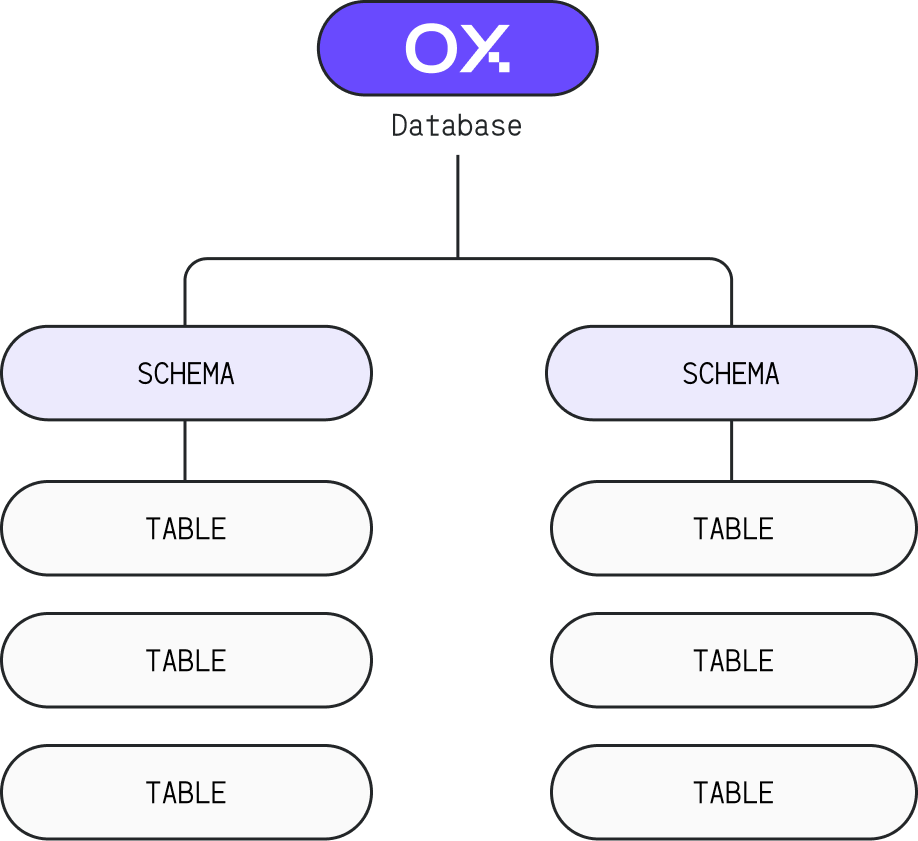
Roles in Oxla can be used to manage access to the following objects: * Database * Schema * Table In Oxla, the terms `role` and `user` are interchangeable and refer to the same concept. In SQL queries, the keywords `ROLE` and `USER` have identical semantics. ## Superusers Oxla includes a default superuser named `oxla`, which always exists and retains superuser rights permanently. Other users may be created as either superusers or non-superusers. This status is set during user creation but can be changed later if needed. Both the default superuser and other superusers have the same permissions. The key difference is that the default superuser cannot be deleted or downgraded to a non-superuser, while other superusers do not have this protection. ## Privileges Required for Role Management All role management operations, such as creating, deleting, listing roles, changing passwords, promoting to superuser or degrading to non-superuser; require **superuser** privileges. The only exception is password changes: every role can change its own password. ## Creating Roles The syntax for role creation is as follows: ```sql theme={null} CREATE ROLE username [ WITH ] PASSWORD 'your_secure_password' [ SUPERUSER | NOSUPERUSER] [ LOGIN ]; ``` Here's the breakdown of the above statement: * `username`: name of the role you want to create * `your_secure_password`: the role’s password (required and cannot be empty) * `SUPERUSER` / `NOSUPERUSER`: sets superuser status; defaults to `NOSUPERUSER` * `WITH`: optional clause, no effect on behavior * `LOGIN`: optional clause, included for compatibility; all roles can log in by default The order of `PASSWORD`, `SUPERUSER` / `NOSUPERUSER` and `LOGIN` is flexible. For example: ```sql theme={null} CREATE ROLE username WITH LOGIN SUPERUSER PASSWORD 'your_secure_password'; ``` ## Deleting Roles Roles can own objects and hold privileges. To delete a role, you must first delete or reassign all owned objects and revoke any granted privileges (default privileges do not require revocation). Role can be deleted (dropped) using the following syntax: ```sql theme={null} DROP ROLE username; ``` You cannot delete the user you are currently logged in as. However, you can delete other users even if they are currently connected to the database. Alternatively, one can also execute the following command (PostgreSQL compatibility): ```sql theme={null} DROP USER username; ``` * `username`: name of the role to drop ## Listing Roles To list roles in Oxla, execute the following query: ```sql theme={null} SELECT id, name, user_kind FROM oxla_internal.oxla_role; ``` Example output showing role IDs, names and user kinds: ```text theme={null} id | name | user_kind ----+--------+----------- 1 | oxla | 1 2 | alice | 2 3 | bob | 2 4 | charlie| 3 ``` Column `user_kind` holds one of three possible values: * `1`: default superuser * `2`: regular superuser * `3`: non-superuser ## Modifying Roles Modify roles using `ALTER ROLE` to change passwords or superuser status. Modifying a role does not affect privileges or ownership. ### Changing password Role's password can be changed either by a superuser or a role itself by executing the code below: ```sql theme={null} ALTER ROLE username [ WITH ] PASSWORD 'new_password'; ``` Here's the breakdown of the above syntax: * `username`: name of the role for which you want to change the password, or keyword CURRENT\_ROLE/CURRENT\_USER * `new_password`: new password for that role * `WITH`: optional clause, no effect on behavior ### Promoting to superuser / Demoting to non-superuser Promote a non-superuser to superuser by executing this query: ```sql theme={null} ALTER ROLE username [ WITH ] SUPERUSER; ``` Demote a superuser to non-superuser by executing this query: ```sql theme={null} ALTER ROLE username [ WITH ] NOSUPERUSER; ``` * `username`: role name ### Changing Password and Superuser Status in One Query Change password and superuser status simultaneously by executing this query: ```sql theme={null} ALTER ROLE username [ WITH ] SUPERUSER PASSWORD 'new_password'; ``` --- # Source: https://docs.oxla.com/sql-reference/sql-functions/math-functions/round.md > ## Documentation Index > Fetch the complete documentation index at: https://docs.oxla.com/llms.txt > Use this file to discover all available pages before exploring further. # ROUND ## Overview The `ROUND()` function rounds numbers using round half to even method (bankers rounding). ## Syntax The following illustrates the syntax of the `ROUND()` function: ```sql theme={null} ROUND(number); ``` Where: * `number`: The number to round, it can be positive, negative, or zero, and it can be an [Integer](/sql-reference/sql-data-types/numeric-type/numeric) or a [Double Precision](/sql-reference/sql-data-types/numeric-type/numeric). ## **Examples** Let's explore some examples to see how the `ROUND()` function works. ### Case #1: **Basic Usage** In this example, we round decimal numbers to integers: ```sql theme={null} SELECT round(28.11) AS "round(28.11)", round(12.51) AS "round(12.51)", round(-9.11) AS "round(-9.11)", round(102.5) AS "round(102.5)", round(101.5) AS "round(101.5)", round(-40.51) AS "round(-40.51)"; ``` The query will return the nearest integer for all provided values. ```sql theme={null} round(28.11) | round(12.51) | round(-9.11) | round(102.5) | round(101.5) | round(-40.51) --------------+--------------+--------------+--------------+---------------+--------------- 28 | 13 | -9 | 102 | 102 | -41 ``` ### Case #2: Using `ROUND` with Table Suppose you have a table named **Product** that stores product prices with multiple decimal places. You want to round the prices. ```sql theme={null} CREATE TABLE Product ( ProductID INT, ProductName TEXT, Price DOUBLE PRECISION ); INSERT INTO Product (ProductID, ProductName, Price) VALUES (1, 'Widget A', 12.345), (2, 'Widget B', 34.678), (3, 'Widget C', 9.99), (4, 'Widget D', 45.00), (5, 'Widget E', 7.12345), (6, 'Widget F', 19.876), (7, 'Widget G', 3.5), (8, 'Widget H', 29.999); ``` We use the `ROUND()` function to round the Price column when retrieving the data. ```sql theme={null} SELECT ProductName, ROUND(Price) AS RoundedPrice FROM Product; ``` The result will display the product names along with their prices rounded. ```sql theme={null} productname | roundedprice -------------+-------------- Widget A | 12 Widget B | 35 Widget C | 10 Widget D | 45 Widget E | 7 Widget F | 20 Widget G | 4 Widget H | 30 ``` --- # Source: https://docs.oxla.com/sql-reference/sql-functions/window-functions/row-number.md > ## Documentation Index > Fetch the complete documentation index at: https://docs.oxla.com/llms.txt > Use this file to discover all available pages before exploring further. # ROW_NUMBER ## Overview The `ROW_NUMBER()` window function returns the number of the current row within its partition (counting from 1), based on the `ORDER BY` expression in the `OVER` clause. It can be used with all data types supported by Oxla. ## Syntax The syntax for this function is as follows: ```sql theme={null} ROW_NUMBER() OVER ( [PARTITION BY partition_expression, ... ] ORDER BY sort_expression [ASC | DESC], ... ) ``` The output's type for this function is `BIGINT`. Rows with equal values for the `ORDER BY` expression receive different row numbers nondeterministically. ## Parameters * `()`: this function takes no arguments but parentheses is required ## Examples For the needs of this section, we will create the `winsales` table that stores details about some sales transactions: ```sql theme={null} CREATE TABLE winsales( salesid int, dateid date, sellerid int, buyerid text, qty int, qty_shipped int); INSERT INTO winsales VALUES (30001, '8/2/2003', 3, 'b', 10, 10), (10001, '12/24/2003', 1, 'c', 10, 10), (10005, '12/24/2003', 1, 'a', 30, null), (40001, '1/9/2004', 4, 'a', 40, null), (10006, '1/18/2004', 1, 'c', 10, null), (20001, '2/12/2004', 2, 'b', 20, 20), (40005, '2/12/2004', 4, 'a', 10, 10), (20002, '2/16/2004', 2, 'c', 20, 20), (30003, '4/18/2004', 3, 'b', 15, null), (30004, '4/18/2004', 3, 'b', 20, null), (30007, '9/7/2004', 3, 'c', 30, null); ``` ### ROW\_NUMBER() with ORDER BY In this example, we will focus on executing the `ROW_NUMBER()` function with `ORDER BY` keyword, assign a row number to each row and order the table by the row number (the results will be sorted after the window function results are applied): ```sql theme={null} SELECT salesid, qty ROW_NUMBER() OVER (ORDER BY salesid) FROM winsales ORDER BY 3; ``` Here is the output for the code above: ```sql theme={null} salesid | qty | row_number ---------+-----+------------ 10001 | 10 | 1 10005 | 30 | 2 10006 | 10 | 3 20001 | 20 | 4 20002 | 20 | 5 30001 | 10 | 6 30003 | 15 | 7 30004 | 20 | 8 30007 | 30 | 9 40001 | 40 | 10 40005 | 10 | 11 (11 rows) ``` ### ROW\_NUMBER() with ORDER BY and PARTITION BY In this example, we will focus on executing the `ROW_NUMBER()` function with `ORDER BY` keyword and `PARTITION BY` clause, partition the table by seller ID, assign a row number to each row and order the table by the sales ID and row number (the results will be sorted after the window function results are applied): ```sql theme={null} SELECT salesid, sellerid, qty ROW_NUMBER() OVER (PARTITION BY sellerid ORDER BY salesid) FROM winsales ORDER BY 1; ``` The output of the code above will be as follows: ```sql theme={null} salesid | sellerid | qty | row_number ---------+----------+-----+------------ 10001 | 1 | 10 | 1 10005 | 1 | 30 | 2 10006 | 1 | 10 | 3 20001 | 2 | 20 | 1 20002 | 2 | 20 | 2 30001 | 3 | 10 | 1 30003 | 3 | 15 | 2 30004 | 3 | 20 | 3 30007 | 3 | 30 | 4 40001 | 4 | 40 | 1 40005 | 4 | 10 | 2 (11 rows) ``` ### Time Series: Assigning Sequential Row Numbers by Date In this example, we will assign a sequential row number to each sale ordered by `dateid`: ```sql theme={null} SELECT dateid, salesid, qty, ROW_NUMBER() OVER (ORDER BY dateid, salesid) AS time_series_position FROM winsales ORDER BY dateid, salesid; ``` By executing the query above, we will get the following output: ```sql theme={null} dateid | salesid | qty | time_series_position ------------+---------+-----+---------------------- 2003-08-02 | 30001 | 10 | 1 2003-12-24 | 10001 | 10 | 2 2003-12-24 | 10005 | 30 | 3 2004-01-09 | 40001 | 40 | 4 2004-01-18 | 10006 | 10 | 5 2004-02-12 | 20001 | 20 | 6 2004-02-12 | 40005 | 10 | 7 2004-02-16 | 20002 | 20 | 8 2004-04-18 | 30003 | 15 | 9 2004-04-18 | 30004 | 20 | 10 2004-09-07 | 30007 | 30 | 11 (11 rows) ``` --- # Source: https://docs.oxla.com/sql-reference/schema.md > ## Documentation Index > Fetch the complete documentation index at: https://docs.oxla.com/llms.txt > Use this file to discover all available pages before exploring further. # Schema Definition ## What is Schema? Have you ever wondered how to work with your fellows in one database without interfering with each other? Is it possible to organize the database objects into logical groups which do not collide with the other objects' names? We can do those things with **Schema**: A **schema** is a collection of tables. A schema also contains views, indexes, sequences, data types, operators, and functions. We support multiple schemas. For example, you can have a database named `oxla` and have multiple schemas based on your needs, like `auth`, `model`, `business`, etc. ## 
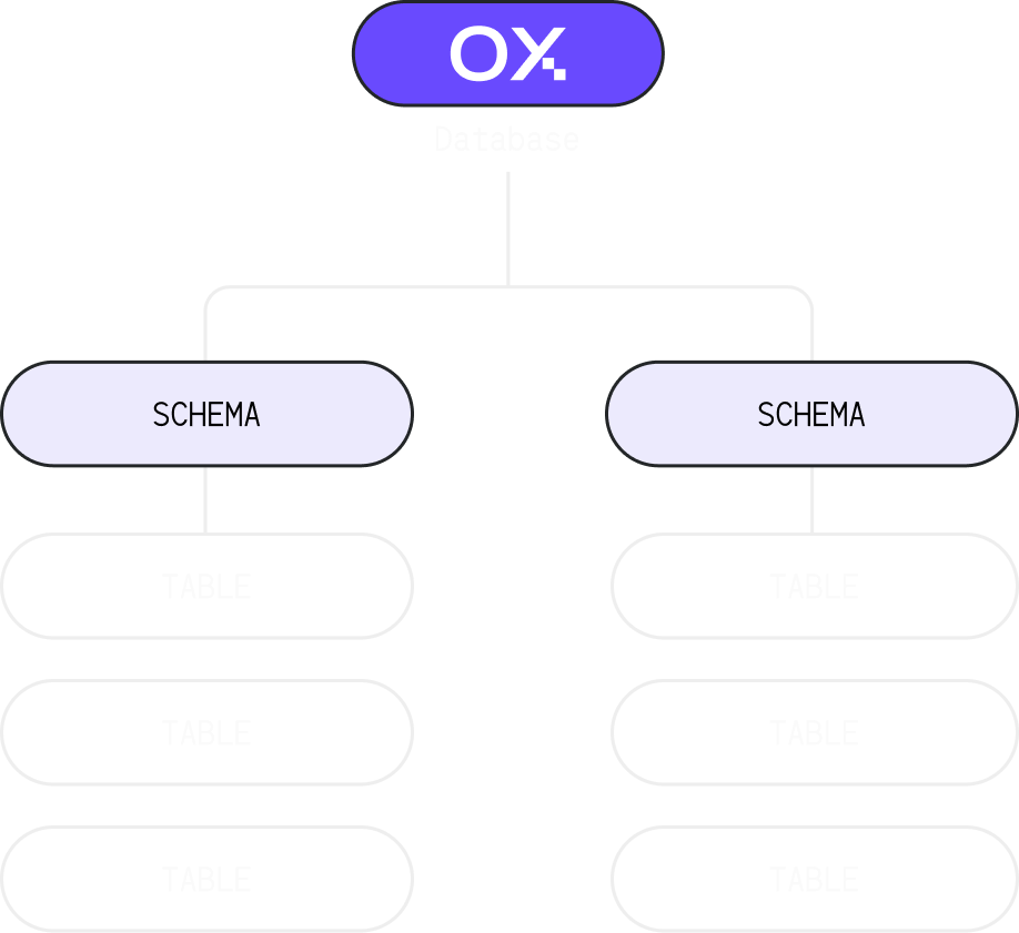
Default Schema in Oxla By default, the `public` schema is used in Oxla. When unqualified `table_name` is used, that `table_name` is equivalent to `public.table_name`. It also applies to `CREATE`, `DROP`, and `SELECT TABLE` statements. Furthermore, you can create multiple schemas per your needs. ## Schema Usage Scenarios ### 1. Create a Schema The basic syntax of creating a schema is as follows: ```sql theme={null} CREATE SCHEMA [IF NOT EXISTS] schema_name; ``` * `schema_name` is the schema name you are going to create. * `IF NOT EXISTS` is an optional parameter to avoid errors if the schema already exists. ### 2. Create a Table in Schema The syntax to create a table in a specified schema is as follows: ```sql theme={null} CREATE TABLE schema_name.table_name( ... ); ``` * `schema_name` is the schema that you have created. * `table_name` is the table name you are going to create. ### 3. Select a Table in Schema After creating the table and inserting some data, display all rows with the syntax below: ```sql theme={null} SELECT * FROM schema_name.table_name; ``` * `schema_name` is the name of the schema. * `table_name` is the name of the table you want to display. ### 4. Drop the Schema **Option 1**: To drop an empty schema where no objects remain in it, use the command below: ```sql theme={null} DROP SCHEMA [IF EXISTS] schema_name; ``` * `schema_name` is the schema name you are going to create. * `IF EXISTS` is an optional parameter to avoid errors if the schema does not exist. **Option 2**: Tables reside in a schema, so it is impossible to drop a schema without also dropping the tables. With the command below, you will also drop the schema with the tables. ```sql theme={null} DROP SCHEMA schema_name CASCADE; ``` ## Examples ### Creating Schema 1. First, connect to Oxla and create a schema as shown below: ```sql theme={null} CREATE SCHEMA oxlarefs; ``` 2. Next, create a table in the above schema with the following details: ```sql theme={null} CREATE TABLE oxlarefs.functions( id int, function_name text, active bool ); INSERT INTO oxlarefs.functions(id, function_name, active) VALUES ('1111', 'Numeric', 'TRUE'), ('2222', 'Text', 'TRUE'), ('3333', 'Timestamp', 'TRUE'), ('4444', 'JSON', 'TRUE'), ('5555', 'Boolean', 'TRUE'); ``` 3. You can verify and show the table made with the command below: ```sql theme={null} SELECT * FROM oxlarefs.functions; ``` 4. You will get the following result: ```sql theme={null} +------+---------------+---------+ | id | function_name | active | +------+---------------+---------+ | 1111 | Numeric | t | | 2222 | Text | t | | 3333 | Timestamp | t | | 4444 | JSON | t | | 5555 | Boolean | t | +------+---------------+---------+ ``` ### Creating Schema Using IF NOT EXISTS To avoid errors when the schema already exists, use the `IF NOT EXISTS` option. Here is how it works: #### Example without IF NOT EXISTS 1. First, create the schema without using the `IF NOT EXISTS` option. ```sql theme={null} CREATE SCHEMA oxladb; ``` Output: ```sql theme={null} CREATE SCHEMA ``` 2. If you attempt to create the schema again without using `IF NOT EXISTS`, it will result in an error. ```sql theme={null} CREATE SCHEMA oxladb; ``` Output: ```sql theme={null} ERROR: Schema: oxladb already exists ``` #### Example with IF NOT EXISTS Now, create the schema using the `IF NOT EXISTS` option to avoid the error. ```sql theme={null} CREATE SCHEMA IF NOT EXISTS oxladb; ``` Using `IF NOT EXISTS` allows the query to create a schema even if it already exists. ```sql theme={null} CREATE ``` ### Dropping Schema Use the command below to delete the schema and also the tables in it. ```sql theme={null} DROP SCHEMA oxlarefs CASCADE; ``` Another case is if there is no table or object created inside the schema, you can use the following command to drop the schema. ```sql theme={null} DROP SCHEMA oxlarefs; ``` ### Dropping Schema using IF EXISTS #### Example without IF EXISTS 1. First, drop the schema without using the `IF EXISTS` option. ```sql theme={null} DROP SCHEMA oxladb; ``` Output: ```sql theme={null} DROP ``` 2. If you attempt to drop the schema again without using `IF EXISTS`, it will result in an error. ```sql theme={null} DROP SCHEMA oxladb; ``` Output: ```sql theme={null} ERROR: schema "oxladb" does not exist ``` #### Example with IF EXISTS Now, drop the schema using the `IF EXISTS` option. ```sql theme={null} DROP SCHEMA IF EXISTS oxladb; ``` Using `IF` EXISTS allows the query to succeed even if the schema does not exist. ```sql theme={null} DROP ``` --- # Source: https://docs.oxla.com/sql-reference/sql-statements/select.md > ## Documentation Index > Fetch the complete documentation index at: https://docs.oxla.com/llms.txt > Use this file to discover all available pages before exploring further. # SELECT ## Overview The `SELECT` statement helps you obtain the data you need from one or more tables. The application of this statement will be helpful in several cases listed below: * Evaluating data from only particular fields in a table. * Reviewing data from several tables at the same time. * Retrieving the data based on specific criteria. ## Syntax To request data from a table using the `SELECT` statement, you can use the following syntax: ```sql theme={null} SELECT * FROM table_name; ``` You are allowed to filter the table by column. Refer to the syntax below. ```sql theme={null} SELECT column1, column2, ... FROM table_name; ``` We will define each syntax as follows. * `SELECT` determines the data we need from the database or a table. * `*` referred to as ***select star*** or ***asterisk*** or represents ***all***. It defines that the query should return all columns of the queried tables. * `FROM` clause indicates the table(s) to retrieve data from. * `table_name` represents the table(s) name. * `column1, column2, ...` these are used to specify the columns from where we want to retrieve the data. The `SELECT` statement is case insensitive, which means `select` **or** `SELECT` has the same result. ## Examples We have a table named **student\_data** that stores the id, name, and where the student lives. ```sql theme={null} CREATE TABLE student_data ( id int, name text, domicile text ); INSERT INTO student_data (id, name, domicile) VALUES (119291,'Jordan','Los Angeles'), (119292,'Mike','Melbourne'), (119293,'Will','Sydney'); ``` All the examples below are executed in the `public` schema. You can also display table from another specific schema. Click [here](/sql-reference/schema) for more info. ### Case #1: Query data from all columns 1. In the first case, we want to display all the data from the **student\_data** table. Please refer to the syntax below: ```sql theme={null} SELECT * FROM table_name; ``` 2. Use the `SELECT` statement within the table name to get all the data: ```sql theme={null} SELECT * FROM student_data; ``` 3. If you have successfully run the query, you will get all the data from the **student\_data** table. ```sql theme={null} +--------+----------+----------------+ | id | name | domicile | +--------+----------+----------------+ | 119291 | Jordan | Los Angeles | | 119292 | Mike | Melbourne | | 119293 | Will | Sydney | +--------+----------+----------------+ ``` ### Case #2: Query data from specific columns 1. We want to get the list of students' names with their IDs. Please refer to the syntax below: ```sql theme={null} SELECT column_1, column_2 FROM table_name; ``` 2. Run the following query: ```sql theme={null} SELECT id, name FROM student_data; ``` 3. If you have successfully run the query, you will get a list of students' IDs & names from the **student\_data** table. ```sql theme={null} +--------+----------+ | id | name | +--------+----------+ | 119291 | Jordan | | 119292 | Mike | | 119293 | Will | +--------+----------+ ``` ### Case #3: Query data from a specific column with the condition 1. If we have a large number of data, skimming for the desired data will require a long time. We can apply some conditions to the `SELECT` statement. Please refer to the syntax below: ```sql theme={null} SELECT column_1 FROM table_name WHERE condition; ``` 2. Let's say we want to know the student's name who lives in Sydney, have a look and run the query below: ```sql theme={null} SELECT name FROM student_data WHERE domicile='Sydney'; ``` 3. If you have successfully run the query, we now know that Will lives in Sydney. ```sql theme={null} +----------+ | name | +----------+ | Will | +----------+ ``` --- # Source: https://docs.oxla.com/sql-reference/sql-statements/set-show.md > ## Documentation Index > Fetch the complete documentation index at: https://docs.oxla.com/llms.txt > Use this file to discover all available pages before exploring further. # SET/SHOW ## Overview The `SET` statement lets you set specific options while the `SHOW` statement helps you see the current values in Oxla. ## Syntax The syntax for these functions is as follows: ```sql theme={null} SET ```sql theme={null} SHOW The available options that can be set and shown are: * `extra_float_digits`: by default, Oxla displays a limited number of digits, but you can set how many extra digits are displayed after the decimal point in floating-point numbers by using this option * `application_name`: sets a custom name for the application * `timezone`: determines the time zone used for date and time functions * `client_min_messages`: sets the message levels sent to the client (valid values are `DEBUG5`, `DEBUG4`, `DEBUG3`, `DEBUG2`, `DEBUG1`, `LOG`, `NOTICE`, `WARNING` and `ERROR`) * `search_path`: defines namespaces at which Oxla looks for tables * `enable_fast_math`: enables mathematical optimizations that trade precision for speed by utilizing faster, less accurate mathematical functions ## Examples ### SET Statement To change the number of displayed digits for floating-point values, use the `SET` statement in a following way: ```sql theme={null} SET extra_float_digits TO 2; ``` ```sql theme={null} SHOW extra_float_digits; ``` ```sql theme={null} extra_float_digits -------------------- 2 ``` To change the client message, use the `SET` statement as follows: ```sql theme={null} SET client_min_messages TO 'WARNING'; ``` ```sql theme={null} SHOW client_min_messages; ``` ```sql theme={null} client_min_messages --------------------- warning ``` To change the mode of the fast math option, use the `SET` statement like this: ```sql theme={null} SET oxla.enable_fast_math = ON; ``` ```sql theme={null} SHOW oxla.enable_fast_math; ``` ```sql theme={null} oxla_enable_fast_math ----------------------- 1 (1 row) ``` ### SHOW Statement To display the current timezone setting, use the following query: ```sql theme={null} SHOW timezone; ``` ```sql theme={null} timezone ---------- Etc/UTC ``` To display the current search path, run the query below: ```sql theme={null} SHOW search_path; ``` ```sql theme={null} search_path ------------- public ``` To check the status of the fast math option, use the following method: ```sql theme={null} SHOW oxla.enable_fast_math; ``` ```sql theme={null} oxla_enable_fast_math ----------------------- 0 (1 row) ``` --- # Source: https://docs.oxla.com/sql-reference/sql-functions/other-functions/shobj-description.md > ## Documentation Index > Fetch the complete documentation index at: https://docs.oxla.com/llms.txt > Use this file to discover all available pages before exploring further. # shobj_description() ## Overview The shobj\_description() is a comment information function that retrieves the comment associated with a shared database object. ## Syntax The syntax for the `shobj_description()` function is as follows:
shobj\_description (object\_oid, catalog\_name) → NULL
## Parameters The following parameters are required to execute this function: * object\_oid: specifies the object identifier (OID) of the shared object for which you want to retrieve the comment * catalog\_name: specifies the name of the system catalog that contains the shared object ## Restrictions * This function always returns `NULL` if there are no parameters specified --- # Source: https://docs.oxla.com/sql-reference/sql-statements/show-nodes.md > ## Documentation Index > Fetch the complete documentation index at: https://docs.oxla.com/llms.txt > Use this file to discover all available pages before exploring further. # SHOW NODES ## Overview The `SHOW NODES` statement returns the current state of the cluster and is only available to the superuser. It is not case-sensitive, so `show nodes`, `Show Nodes`, and `SHOW NODES` do the same thing ## Example To view the current cluster state, you need to execute the following command: ```sql theme={null} SHOW NODES; ``` Once it's done, you'll see a table with the information about each node in the cluster, in a following way: ```sql theme={null} name | election_state | followers_count | connected_nodes_count | degradation_error ---------------+-----------------+-----------------+-----------------------+------------------- n_oxla_node_1 | LEADER_FOLLOWER | 0 | 3 | n_oxla_node_3 | LEADER | 3 | 3 | n_oxla_node_2 | LEADER_FOLLOWER | 0 | 3 | (3 rows) ``` Each row represents the state of an individual node within the cluster, where: * `name`: name of the node * `election_state`: current state of the node (e.g. `LEADER`) * `followers_count`: number of nodes following the leader, which applies to the leader node * `connected_nodes_count`: total number of nodes connected, including itself * `degradation_error`: error message if the node is not working correctly, otherwise it shows `NULL` --- # Source: https://docs.oxla.com/sql-reference/sql-statements/show-tables.md > ## Documentation Index > Fetch the complete documentation index at: https://docs.oxla.com/llms.txt > Use this file to discover all available pages before exploring further. # SHOW TABLES ## Overview The `SHOW TABLES` statement allows you to obtain information about existing tables. It only shows tables in schemas, on which a user has the `USAGE` grant ## Example So as to list all available tables, you need to execute the following query: ```sql theme={null} SHOW TABLES; ``` This will produce an output with a list of all existing tables, an example of which is presented below: ```sql theme={null} +------------+ | name | +------------+ | lineorder | | part | | customer | | supplier | +------------+ ``` --- # Source: https://docs.oxla.com/sql-reference/sql-functions/math-functions/sign.md > ## Documentation Index > Fetch the complete documentation index at: https://docs.oxla.com/llms.txt > Use this file to discover all available pages before exploring further. # SIGN ## Overview The `SIGN()` function returns a sign of an argument. The returned values are -1 if the argument is less than zero, 1 if the argument is greater than zero, 0 if the argument is equal to zero. ## Syntax The syntax for the `SIGN() `function is as follows: ```sql theme={null} SIGN(x) ``` The `SIGN()` function requires one argument: * `x`: an expression that evaluates to a number. ## Examples ### Case #1: Sign of a number The following example demonstrates how the `SIGN()` function can be used to obtain the sign of a number: ```sql theme={null} SELECT SIGN(0.1) AS "SIGN(0.1)", SIGN(999) AS "SIGN(999)", SIGN(0) AS "SIGN(0)", SIGN(-0) AS "SIGN(-0)"; ``` The query will return the signs of the passed arguments: ```sql theme={null} SIGN(0.1) | SIGN(999) | SIGN(0) | SIGN(-0) -----------+-----------+---------+---------- 1 | 1 | 0 | 0 ``` Note: `-0` is accepted as an argument and is equal to zero ### Case #2: SIGN() function with an expression The following example demonstrates how the `SIGN()` function can be used with an expression: ```sql theme={null} SELECT SIGN(100 - 200); ``` will return the sign of the expression evaluation: ```sql theme={null} sign ------ -1 ------ ``` ### Case #3: Using the SIGN() function with a table The following example demonstrates how the `SIGN()` function can be used with a table to obtain the absolute values of all numbers in a specific column: 1. Create a table signTable containing an ***value*** column with some positive, negative and equal to zero values: ```sql theme={null} CREATE TABLE signTable(value float); INSERT INTO signTable(value) VALUES (1000), (-200), (0), (0.22), (-12.3), (-0.0); ``` 2. Use the following query to find the sign of all inserted values: ```sql theme={null} SELECT value, SIGN(value) AS sign FROM signTable; ``` 3. The result will be as follows:: ```sql theme={null} value | sign -------+------ 1000 | 1 -200 | -1 0 | 0 0.22 | 1 -12.3 | -1 -0 | 0 ``` --- # Source: https://docs.oxla.com/sql-reference/sql-functions/math-functions/sin.md > ## Documentation Index > Fetch the complete documentation index at: https://docs.oxla.com/llms.txt > Use this file to discover all available pages before exploring further. # SIN ## Overview `SIN()` is a numeric function that returns the trigonometric sine value of a specified angle in radians. ## Syntax The syntax of the `SIN()` function is as follows. ```sql theme={null} SIN (x) ``` The `SIN()` function requires one argument: `x`:  A positive or a negative angle (or an expression that evaluates to an angle). ## Examples ### Case #1: Sine a Positive Value The example below will use the `SIN()` function with a positive angle as the argument. ```sql theme={null} SELECT SIN(5); ``` It will return the sine value of 5. ```sql theme={null} +-----------------------+ | f    | +-----------------------+ | -0.9589242746631385  | +-----------------------+ ``` ### Case #2: Sine a Negative Value The following example shows the `SIN(`) function with a negative angle as the argument. ```sql theme={null} SELECT SIN(-3); ``` The output will be as follows. ```sql theme={null} +----------------------+ | f                 | +----------------------+ | -0.1411200080598672 | +----------------------+ ``` ### Case #3: Sine a Fraction Value The following example shows the `SIN()` function with a fractional value as the argument. ```sql theme={null} SELECT SIN(5.8732); ``` The output will be as follows. ```sql theme={null} +----------------------+ | f                 | +----------------------+ | -0.3985959081271079 | +----------------------+ ``` ### Case #4: Sine With an Expression The `SIN()` function can also include an expression, as shown in the example below: ```sql theme={null} SELECT sin(8.5 * 2.3); ``` You will get the following output: ```sql theme={null} +-----------------------+ | f                 | +-----------------------+ | 0.6445566903363104 | +-----------------------+ ``` ### Case #5: Using the `SIN()` Function With a Table In the following example, we will combine `SIN()` function with `CREATE TABLE` statement to obtain the sine values of a specific column. 1. Create a new table named **sineTable** containing the **initialValue** column. Input some values with the negative and positive angles into the column. ```sql theme={null} CREATE TABLE sineTable(initialValue int); INSERT INTO sineTable(initialValue) VALUES (-5),(18), (0),(-27); ``` 2. Run the query below to get the output of a sine value: ```sql theme={null} SELECT * ,SIN(initialValue) AS sinValue FROM sineTable; ``` 3. The final result will have the **initialValue** column with the source value and the **sinValue** column with their calculated sine values.   ```sql theme={null} +---------------+-------------------------------+ | initialvalue  | sinValue                      | +---------------+-------------------------------+ | -75           | 0.38778163540943045           | | 180           | -0.8011526357338304           | | 0           | 0                             | | -270     | 0.1760459464712114            | +---------------+-------------------------------+ ``` --- # Source: https://docs.oxla.com/sql-reference/sql-functions/math-functions/sqrt.md > ## Documentation Index > Fetch the complete documentation index at: https://docs.oxla.com/llms.txt > Use this file to discover all available pages before exploring further. # SQRT ## Overview The `SQRT()` function returns the square root of a given positive number. ## Syntax The syntax for the `SQRT()` function in Oxla is: ```sql theme={null} SQRT(x) ``` The `SQRT()` function requires one argument: * `x`: A positive number or an expression that evaluates to a positive number. ## Examples ### Case #1: SQRT() a Positive Value The following example demonstrates how the `SQRT()` function can be used to find the square root of a positive integer: ```sql theme={null} SELECT SQRT(81); ``` You will get the following result: ```sql theme={null} +-----+ | f | +-----+ | 9 | +-----+ ``` ### Case #2: SQRT() With an Expression Let’s look at an example of using the `SQRT()` function to find the square root of the result of an expression. ```sql theme={null} SELECT SQRT(60 + 4); ``` The result of the above statement is the square root of 64: ```sql theme={null} +-----+ | f | +-----+ | 8 | +-----+ ``` ### Case #3: SQRT() With Double Precision Result In addition to integers, Oxla also supports calculating square roots with floating-point numbers as the outcome. For further details, please refer to the statement below: ```sql theme={null} SELECT SQRT(70); ``` The output of the statement above is 8.3666, which is the square root of 70 with double precision, as demonstrated below: ```sql theme={null} +----------+ | f | +----------+ | 8.3666 | +----------+ ``` ### Case #4: SQRT() a Negative Number The following example demonstrates how attempting to use the `SQRT()` function with a negative value will return an error: ```sql theme={null} SELECT SQRT(-25); ``` As the `SQRT()` function only accepts positive numbers, you will get a ***NaN (Not a Number)*** result for the square root of -25, as shown below: ```sql theme={null} +-------+ | f | +-------+ | NaN | +-------+ ``` ### Case #5: SQRT Operator (`|/(x)`) Here's an example using the SQRT operator (`|/(x)`) to calculate the square root of a given number: ```sql theme={null} SELECT |/(169) AS sqrt_operator; ``` In this example, we calculate the square root of 169 using the SQRT operator. The result of this query will be: ```sql theme={null} sqrt_operator --------------- 13 ``` --- # Source: https://docs.oxla.com/security/ssl-configuration.md > ## Documentation Index > Fetch the complete documentation index at: https://docs.oxla.com/llms.txt > Use this file to discover all available pages before exploring further. # SSL Configuration Oxla provides support for using SSL connections to encrypt client/server communications for increased security, that safeguards your data. The following documentation will guide you through the process of configuring SSL for your Oxla database. ## SSL Configuration Settings To enable SSL support, the following settings must be correctly configured: * **mode**: `require` or `optional` * **cert\_file**: path to the server's public certificate in PEM format * **key\_file**: path to the server's private key in PEM format Providing a `ca_crt_file`, which is used to verify whether the certificate was signed by the Certificate Authority (CA) is **optional**. The settings for `min_protocol_version` and `max_protocol_version` can be omitted, as they have default values. ## SSL Enabled Configuration (Mode: Optional) Clients are authorized to establish connections using both non-SSL and SSL protocols. Connections established with `sslmode=require` or `sslmode=disable` will be accepted. ```yaml theme={null} ssl: mode: optional ca_crt_file: "path/to/ca.crt" cert_file: "path/to/ssl.crt" key_file: "path/to/ssl.key" min_protocol_version: 1.2 # Minimum supported SSL version, supported values: 1.2, 1.3 max_protocol_version: 1.3 # Maximum supported SSL version, supported values: 1.2, 1.3 ``` ## SSL Enabled Configuration (Mode: Require) Clients are permitted to connect only through SSL connections. Any attempts to establish a connection using tools that require SSL, such as `psql` with the `sslmode=disable` option, will be rejected. ```yaml theme={null} ssl: mode: require ca_crt_file: "path/to/ca.crt" cert_file: "path/to/ssl.crt" key_file: "path/to/ssl.key" min_protocol_version: 1.2 # Minimum supported SSL version, supported values: 1.2, 1.3 max_protocol_version: 1.3 # Maximum supported SSL version, supported values: 1.2, 1.3 ``` ### SSL Disabled Configuration Clients are permitted to connect only through non-SSL connections. Any attempts to establish a connection using tools that require SSL, such as `psql` with the `sslmode=require` option, will be rejected. ```yaml theme={null} ssl: mode: off ``` ## SSL Modes Description Table | SSL Mode | Eavesdropping Protection | Support | | :------: | :----------------------: | :-------------------------------------------- | | off | No | SSL connections not supported | | require | Yes | Only SSL connections are allowed | | optional | Yes | both SSL and no SSL connections are supported | ## Examples of SSL Configuration For a more detailed explanation of the configuration options, please refer to the Oxla Configuration File. --- # Source: https://docs.oxla.com/sql-reference/sql-functions/string-functions/starts-with.md > ## Documentation Index > Fetch the complete documentation index at: https://docs.oxla.com/llms.txt > Use this file to discover all available pages before exploring further. # STARTS_WITH ## Overview The `STARTS_WITH()` function determines whether the first argument starts with a specified string in the second argument or not. ```sql theme={null} STARTS_WITH(first_argument, 'second_argument') ``` * `first_argument`: the specified argument, which will be the search reference. It can be a string or a column name. * `second_argument`: the specified argument, which will have the search keywords. The input type will be `STRING`, and the return type is `BOOL`, shown as `true` or `false`. Special case: * It will return `NULL` for the `NULL` record. * It will return `true` (including the `NULL` record) if the `second_argument` is not specified. ## Examples ### Case 1: `STARTS_WITH()` function using column Let’s say we have a table with the title **petsData**, as shown below. ```sql theme={null} CREATE TABLE petsData ( petid int, petname text, species text, breed text, sex text, age int ); INSERT INTO petsData (petid, petname, species, breed, sex, age) VALUES (2021001,'Bartholomeow','cat','persian','m',2), (2021004,'Jack','dog','boston terrier','m',1), (2022001,'Jesse','hamster','dzungarian','m',1), (2022010,'Bella','dog','dobberman','f',3), (2022011,'June','cat','american shorthair','f',2); ``` ```sql theme={null} SELECT * FROM petsData; ``` The above query will show the following table: ```sql theme={null} +----------+--------------+----------+---------------------+------+-----+ | petid | petname | species | breed | sex | age | +----------+--------------+----------+---------------------+------+-----+ | 2021001 | Bartholomeow | cat | persian | m | 2 | | 2021004 | Jack | dog | boston terrier | m | 1 | | 2022001 | Jesse | hamster | dzungarian | m | 1 | | 2022010 | Bella | dog | dobberman | f | 3 | | 2022011 | June | cat | american shorthair | f | 2 | +----------+--------------+----------+---------------------+------+-----+ ``` From the table above, we want to retrieve the values of **petname** column that start with “J” by using the following query: ```sql theme={null} SELECT petname, STARTS_WITH(petname, 'J') FROM petsData; ``` It will return `true` to the pet with a pet starting with the letter J. Otherwise, `false`. ```sql theme={null} +--------------+---------------+ | petname | starts_with | +---------------+--------------+ | Bartholomeow | false | | Jack | true | | Jesse | true | | Bella | false | | June | true | +---------------+--------------+ ``` ### Case 2: `STARTS_WITH()` function with no specified argument Here we have the **petsData** table with a `NULL` value in the breed column. ```sql theme={null} CREATE TABLE petsData ( petid int, petname text, species text, breed text, sex text, age int ); INSERT INTO petsData (petid, petname, species, breed, sex, age) VALUES (2021001,'Bartholomeow','cat','persian','m',2), (2021004,'Jack','dog','boston terrier','m',1), (2022001,'Jesse','hamster','dzungarian','m',1), (2022010,'Bella','dog','dobberman','f',3), (2022011,'June','cat','american shorthair','f',2), (2022012,'Phoebe','gold fish','','f',1); ``` ```sql theme={null} SELECT * FROM petsData; ``` ```sql theme={null} +----------+--------------+------------+---------------------+------+------+ | petid | petname | species | breed | sex | age | +----------+--------------+------------+---------------------+------+------+ | 2021001 | Bartholomeow | cat | persian | m | 2 | | 2021004 | Jack | dog | boston terrier | m | 1 | | 2022001 | Jesse | hamster | dzungarian | m | 1 | | 2022010 | Bella | dog | dobberman | f | 3 | | 2022011 | June | cat | american shorthair | f | 2 | | 2022012 | Phoebe | gold fish | | f | 1 | +----------+--------------+------------+---------------------+------+------+ ``` For example, we run the `STARTS_WITH` function but with no specified `second_argument:` ```sql theme={null} SELECT breed, STARTS_WITH(breed, '') FROM petsData; ``` We will have the following result where the `STARTS_WITH` will return true to all records (even the `null` one): ```sql theme={null} +---------------------+--------------+ | breed | starts_with | +---------------------+--------------+ | persian | true | | boston terrier | true | | dzungarian | true | | dobberman | true | | american shorthair | true | | null | true | +---------------------+--------------+ ``` --- # Source: https://docs.oxla.com/sql-reference/sql-functions/aggregate-functions/stddev-pop.md > ## Documentation Index > Fetch the complete documentation index at: https://docs.oxla.com/llms.txt > Use this file to discover all available pages before exploring further. # STDDEV_POP() ## Overview The `STDDEV_POP()` aggregate function calculates the population stardard deviation of a set of numeric values. ## Syntax The syntax for this function is as follows: ```sql theme={null} STDDEV_POP(expression) ``` ## Parameters * `expression`: numeric expression or column for which the population standard deviation is calculated ## Example For the needs of this section, we're going to use a simplified version of the `film` table from the Pagila database, containing only the `title`, `length` and `rating` columns. The complete schema for the `film` table can be found on the Pagila database website. ```sql theme={null} DROP TABLE IF EXISTS film; CREATE TABLE film ( title text NOT NULL, length int, rating int ); INSERT INTO film(title, length, rating) VALUES ('ATTRACTION NEWTON', 83, 5), ('CHRISTMAS MOONSHINE', 150, 7), ('DANGEROUS UPTOWN', 121, 4), ('KILL BROTHERHOOD', 54, 3), ('HALLOWEEN NUTS', 47, 5), ('HOURS RAGE', 122, 7), ('PIANIST OUTFIELD', 136, 7), ('PICKUP DRIVING', 77, 3), ('INDEPENDENCE HOTEL', 157, 7), ('PRIVATE DROP', 106, 4), ('SAINTS BRIDE', 125, 3), ('FOREVER CANDIDATE', 131, 7), ('MILLION ACE', 142, 5), ('SLEEPY JAPANESE', 137, 4), ('WRATH MILE', 176, 7), ('YOUTH KICK', 179, 7), ('CLOCKWORK PARADISE', 143, 5); ``` They query below uses the `STDDEV_POP()` function to calculate the population standard deviation for the `length` column: ```sql theme={null} SELECT STDDEV_POP(length) AS LengthPopStdDev FROM film; ``` By executing the above code, we will get the following output: ```sql theme={null} lengthpopstddev ------------------- 37.23496886764368 (1 row) ``` --- # Source: https://docs.oxla.com/sql-reference/sql-functions/aggregate-functions/stddev-samp.md > ## Documentation Index > Fetch the complete documentation index at: https://docs.oxla.com/llms.txt > Use this file to discover all available pages before exploring further. # STDDEV_SAMP() ## Overview The `STDDEV_SAMP()` aggregate function calculates the sample standard deviation of a set of numeric values. This function measures how much the values deviate from their mean, assuming the data is a sample of a larger population. ## Syntax The syntax for this function is as follows: ```sql theme={null} STDDEV_SAMP(expression) ``` ## Parameters * `expression`: numeric expression or column for which the sample standard deviation is calculated ## Example For the needs of this section, we're going to use a simplified version of the `film` table from the Pagila database, containing only the `title`, `length` and `rating` columns. The complete schema for the `film` table can be found on the Pagila database website. ```sql theme={null} DROP TABLE IF EXISTS film; CREATE TABLE film ( title text NOT NULL, length int, rating int ); INSERT INTO film(title, length, rating) VALUES ('ATTRACTION NEWTON', 83, 5), ('CHRISTMAS MOONSHINE', 150, 7), ('DANGEROUS UPTOWN', 121, 4), ('KILL BROTHERHOOD', 54, 3), ('HALLOWEEN NUTS', 47, 5), ('HOURS RAGE', 122, 7), ('PIANIST OUTFIELD', 136, 7), ('PICKUP DRIVING', 77, 3), ('INDEPENDENCE HOTEL', 157, 7), ('PRIVATE DROP', 106, 4), ('SAINTS BRIDE', 125, 3), ('FOREVER CANDIDATE', 131, 7), ('MILLION ACE', 142, 5), ('SLEEPY JAPANESE', 137, 4), ('WRATH MILE', 176, 7), ('YOUTH KICK', 179, 7), ('CLOCKWORK PARADISE', 143, 5); ``` The query below uses the `STDDEV_SAMP()` function to calculate the sample standard deviation for the `length` column where `rating` is greater than or equal to 4: ```sql theme={null} SELECT STDDEV_SAMP(length) AS LengthSampleStdDev FROM film WHERE rating >= 4; ``` By running the code above we will get the following output: ```sql theme={null} lengthsamplestddev -------------------- 34.92503746251735 (1 row) ``` --- # Source: https://docs.oxla.com/sql-reference/sql-functions/aggregate-functions/stddev.md > ## Documentation Index > Fetch the complete documentation index at: https://docs.oxla.com/llms.txt > Use this file to discover all available pages before exploring further. # STDDEV() ## Overview The `STDDEV()` aggregate function calculates the sample standard deviation of a set of numeric values. Standard deviation measures the dispersion or spread of data points around the mean. ## Syntax The syntax for this function is as follows: ```sql theme={null} STDDEV(expression) ``` ## Parameters * `expression`: numeric expression or column for which the sample standard deviation is calculated ## Example For the needs of this section we're going to use a simplified version of the `film` table from the Pagila database, containing only the `title`, `length` and `rating` columns. The complete schema for the `film` table can be found on the Pagila database website. ```sql theme={null} DROP TABLE IF EXISTS film; CREATE TABLE film ( title text NOT NULL, length int, rating int ); INSERT INTO film(title, length, rating) VALUES ('ATTRACTION NEWTON', 83, 5), ('CHRISTMAS MOONSHINE', 150, 7), ('DANGEROUS UPTOWN', 121, 4), ('KILL BROTHERHOOD', 54, 3), ('HALLOWEEN NUTS', 47, 5), ('HOURS RAGE', 122, 7), ('PIANIST OUTFIELD', 136, 7), ('PICKUP DRIVING', 77, 3), ('INDEPENDENCE HOTEL', 157, 7), ('PRIVATE DROP', 106, 4), ('SAINTS BRIDE', 125, 3), ('FOREVER CANDIDATE', 131, 7), ('MILLION ACE', 142, 5), ('SLEEPY JAPANESE', 137, 4), ('WRATH MILE', 176, 7), ('YOUTH KICK', 179, 7), ('CLOCKWORK PARADISE', 143, 5); ``` This query below uses the `STDDEV()` function to calculate the sample standard deviation for the `length` column: ```sql theme={null} SELECT STDDEV(length) AS LengthStdDev FROM film; ``` By running the above code we will get the following output: ```sql theme={null} lengthstddev ------------------- 38.38092740197003 (1 row) ``` --- # Source: https://docs.oxla.com/sql-reference/sql-functions/string-functions/strpos.md > ## Documentation Index > Fetch the complete documentation index at: https://docs.oxla.com/llms.txt > Use this file to discover all available pages before exploring further. # STRPOS ## Overview The `STRPOS()` is used to return the position from where the substring (the second argument) is matched with the string (the first argument). ```sql theme={null} STRPOS(string, substring) ``` The input and return must be of type `string`. **Special cases:** * Returns `NULL` if there are no input rows or `NULL` values. * If the `substring` is not found in the string, then the `STRPOS()` function will return 0. ## Examples ### Case 1: Basic `STRPOS()` function In the example below, we will find the **ut** (substring) position in the **computer** (string): ```sql theme={null} SELECT STRPOS('computer', 'ut') AS "Position of ut"; ``` We can see that **ut** is located at the fifth character of the **computer**: ```sql theme={null} +-----------------+ | Position of ut | +-----------------+ | 5 | +-----------------+ ``` ### Case 2: STRPOS() function using column We have a **listofwords** table where it stores the word data. ```sql theme={null} CREATE TABLE listofwords ( words text ); INSERT INTO listofwords (words) VALUES ('corral'), ('traditionally'), ('real'), ('communal'), ('challenge'), ('fall'), ('wall'), ('gallop'), ('albatross'); ``` ```sql theme={null} SELECT * FROM listofwords; ``` The above query will show the following table: ```sql theme={null} +----------------+ | words | +----------------+ | corral | | traditionally | | real | | communal | | challenge | | fall | | wall | | gallop | | albatross | +----------------+ ``` The following query will display the words and a position of a specific substring = ‘**al**’ using the `STRPOS()` function: ```sql theme={null} SELECT words, STRPOS(words, 'al') AS "Position of al" FROM listofwords; ``` The result will display the **al** position of different words: ```sql theme={null} +----------------+------------------+ | words | Position of al | +----------------+------------------+ | corral | 5 | | traditionally | 10 | | real | 3 | | communal | 7 | | challenge | 3 | | fall | 2 | | wall | 2 | | gallop | 2 | | albatross | 1 | +----------------+------------------+ ``` --- # Source: https://docs.oxla.com/sql-reference/sql-functions/string-functions/substr.md > ## Documentation Index > Fetch the complete documentation index at: https://docs.oxla.com/llms.txt > Use this file to discover all available pages before exploring further. # SUBSTR ## Overview The `SUBSTR()` function extracts a specific number of characters from a string. ## Syntax The syntax of the function is illustrated below: **2 Arguments** ```sql theme={null} substr( string, start_position) ``` **3 Arguments** ```sql theme={null} substr( string, start_position, length ) ``` Both syntaxes will have input and return of type `string`. ### Start Position The `start_position` is used as the starting position, specifying the part from where the substring is to be returned. It is written as an integer value. | **Input** | **Return** | | ---------------------------------------------- | ------------------------------------------------------------------------------------------------------------------------------------------------------------------------------------------------------------------------------------------------------------------------------------------------ | | `start_position < 0 ``start_position < string` | The `start_position` is a given character in the string. The count starts from the first character. | | `start_position > string` | Returns an empty substring. | | `start_position` = negative value | The count starts from the provided negative value, with subsequent characters yielded as it approaches 0.

If the index is less than or equal to 0, no characters are returned.

Once it exceeds 0, characters from the string are yielded, starting from the first one. | ### Length The `length` is used to determine the number of characters to be extracted\*. \*It can be one or more characters. | **Input** | **Return** | | ------------------------- | ---------------------------------------------------------------------------------------------------------- | | `length` = 0 | Returns an empty substring. | | `length` is not set | The function will start from the specified `start_position` and end at the last character of the `string`. | | `length` = negative value | Returns an error. | ## Examples ### Case 1: `SUBSTR()` function with specified `start_position` & `length` In this example, we will set the `start_position` with the first six characters and have five characters extracted: ```sql theme={null} SELECT substr('Watermelon',6,5) AS "Fruit"; ``` The updated table is shown below: ```sql theme={null} Fruit ------- melon ``` ### Case 2: `SUBSTR()` function with `length` = 0 The following query will extract a string with `length` = 0: ```sql theme={null} SELECT substr('Watermelon',6,0) AS "Fruit"; ``` It will display an empty output as there is no `length` specified: ```sql theme={null} Fruit ------- ``` ### Case 3: `SUBSTR()` function with `length` = negative value Here we will check if the `length` is specified with a negative value: ```sql theme={null} SELECT substr('Watermelon',6,-2) AS "Fruit"; ``` Instead of extracting the string from the last characters, it will return an error as seen below: ```sql theme={null} ERROR: Length of substring cannot be negative ``` ### Case 4: `SUBSTR()` function with `start_position` > `string` We know that **Watermelon** only has ten characters, but this time, we will figure out if the specified `start_position` is larger than the string’s characters: ```sql theme={null} SELECT substr('Watermelon',20,2) AS "Fruit"; ``` It will display an empty output as shown below: ```sql theme={null} Fruit ------- ``` ### Case 5: `SUBSTR()` Function with 2 Arguments In this example, we will set the `start_position` with the first six characters and have five characters extracted. ```sql theme={null} SELECT substr('database', 6) AS "Result"; ``` It will display the substring from position 6 output as shown below: ```sql theme={null} Result -------- ase ``` --- # Source: https://docs.oxla.com/sql-reference/sql-functions/string-functions/substring.md > ## Documentation Index > Fetch the complete documentation index at: https://docs.oxla.com/llms.txt > Use this file to discover all available pages before exploring further. # SUBSTRING SUBSTR is an alias for SUBSTRING. Learn more at [SUBSTR](/sql-reference/sql-functions/string-functions/substr) documentation. ## Overview The SUBSTRING() function lets you extract a part of a string and return that substring. ## Syntax Here are the 2 basic syntaxes of the `SUBSTRING()` function in Oxla: **2 Arguments** ```sql theme={null} SUBSTRING( string, start_position ) ``` **3 Arguments** ```sql theme={null} SUBSTRING(string, start_position, length) ``` Both syntaxes will have input and return of type `string`. ## Example The following example uses the `SUBSTRING()` function to extract the first 7 characters from the string. ```sql theme={null} SELECT SUBSTRING('OxlaDocumentation', 1, 7); ``` It will display the substring from position 6 output as shown below: ```sql theme={null} substring ----------- OxlaDoc ``` --- # Source: https://docs.oxla.com/sql-reference/sql-functions/window-functions/sum.md # Source: https://docs.oxla.com/sql-reference/sql-functions/aggregate-functions/sum.md > ## Documentation Index > Fetch the complete documentation index at: https://docs.oxla.com/llms.txt > Use this file to discover all available pages before exploring further. # SUM ## Overview `SUM()` calculates the sum of values from stored records. `SUM()` doesn’t consider `NULL` in the calculation, and it returns `NULL` instead of zero if the executed statement returns no rows. The input and return types we support can be seen in the table below. | Input type | Return type | | ---------- | ----------- | | INT | LONG | | LONG | LONG | | FLOAT | DOUBLE | | DOUBLE | DOUBLE | | INTERVAL | INTERVAL | If the input type is 32-bit, then the result will be 64-bit. ## Examples We have two sample tables here: **customer table** ```sql theme={null} CREATE TABLE customer ( customer_id int, cust_name text ); INSERT INTO customer (customer_id, cust_name) VALUES (11112, 'Alex'), (11113, 'Aaron'), (11114, 'Alice'), (11115, 'Nina'), (11116, 'Rosy'), (11117, 'Martha'), (11118, 'John'); ``` ```sql theme={null} SELECT * FROM customer; ``` It will create a table as shown below: ```sql theme={null} +-------------+-----------+ | customer_id | cust_name | +-------------+-----------+ | 11112 | Alex | | 11113 | Aaron | | 11114 | Alice | | 11115 | Nina | | 11116 | Rosy | | 11117 | Martha | | 11118 | John | +-------------+-----------+ ``` **rental table** ```sql theme={null} CREATE TABLE rental ( rental_id int, rental_date timestamp, return_date timestamp, car text, customer_id int, total_price int ); INSERT INTO rental (rental_id, rental_date, return_date, car, customer_id, total_price) VALUES (8557411, '2022-04-02 09:10:19', '2022-04-10 10:15:05', 'Audi', 11112, 1400), (8557421, '2022-04-06 07:00:30', '2022-04-19 07:10:19', 'BMW', 11115, 2000), (8557451, '2022-04-19 08:00:20', '2022-04-24 08:05:00', 'Cadillac', 11112, 1000), (8557311, '2022-05-11 09:15:28', '2022-05-18 09:00:18', 'Audi', 11115, 1500), (8557321, '2022-05-20 10:12:22', '2022-05-28 10:08:48', 'Audi', 11113, 1500), (8557351, '2022-06-10 12:18:09', '2022-06-20 18:12:23', 'Cadillac', 11114, 1200), (8557221, '2022-06-17 14:02:02', '2022-06-20 14:17:02', 'Chevrolet', 11112, 1300), (8557251, '2022-07-12 05:19:49', '2022-07-19 07:15:28', 'Chevrolet', 11116, 1400), (8557231, '2022-08-09 09:29:08', '2022-08-24 09:30:58', 'Cadillac', 11114, 2000), (8557291, '2022-08-18 15:15:20', '2022-09-01 15:30:19', 'BMW', 11117, 3000); ``` ```sql theme={null} SELECT * FROM rental; ``` Here, we have a rental table which stores the details for car rental: ```sql theme={null} +------------+---------------------+---------------------+-----------+---------------+-------------+ | rental_id | rental_date | return_date | car | customer_id | total_price | +------------+---------------------+---------------------+-----------+---------------+-------------+ | 8557411 | 2022-04-02 09:10:19 | 2022-04-10 10:15:05 | Audi | 11112 | 1400 | | 8557421 | 2022-04-06 07:00:30 | 2022-04-19 07:10:19 | BMW | 11115 | 2000 | | 8557451 | 2022-04-19 08:00:20 | 2022-04-24 08:05:00 | Cadillac | 11112 | 1000 | | 8557311 | 2022-05-11 09:15:28 | 2022-05-18 09:00:18 | Audi | 11115 | 1500 | | 8557321 | 2022-05-20 10:12:22 | 2022-05-28 10:08:48 | Audi | 11113 | 1500 | | 8557351 | 2022-06-10 12:18:09 | 2022-06-20 18:12:23 | Cadillac | 11114 | 1200 | | 8557221 | 2022-06-17 14:02:02 | 2022-06-20 14:17:02 | Chevrolet | 11112 | 1300 | | 8557251 | 2022-07-12 05:19:49 | 2022-07-19 07:15:28 | Chevrolet | 11116 | 1400 | | 8557231 | 2022-08-09 09:29:08 | 2022-08-24 09:30:58 | Cadillac | 11114 | 2000 | | 8557291 | 2022-08-18 15:15:20 | 2022-09-01 15:30:19 | BMW | 11117 | 3000 | +------------+---------------------+---------------------+-----------+---------------+-------------+ ``` ### #Case 1: `SUM()` in `SELECT` statement The following example uses the `SUM()` function to calculate the total rent price of all `rental_id`: ```sql theme={null} SELECT SUM (total_price) AS total FROM rental ``` It will return a sum value of the `total_price`: ```sql theme={null} +--------+ | total | +--------+ | 16300 | +--------+ ``` ### #Case 2: `SUM()` with a `NULL` result The following example uses the `SUM()` function to calculate the total rent price of the `customer_id = 11118.` ```sql theme={null} SELECT SUM (total_price) AS total FROM rental WHERE customer_id = 11118; ``` Since no records in the **rental** table have the `customer_id = 11118`, the `SUM()` function returns a `NULL`. ```sql theme={null} +--------+ | total | +--------+ | null | +--------+ ``` ### #Case 3: `SUM()` with `GROUP BY` clause You can use the `GROUP BY` clause to group the records in the table and apply the `SUM()` function to each group afterward. The following example uses the `SUM()` function and the `GROUP BY` clause to calculate the total price paid by each customer: ```sql theme={null} SELECT customer_id, SUM (total_price) AS total_spend FROM rental GROUP BY customer_id; ``` It will calculate the `total_price` from a group of `customer_id` as shown below: ```sql theme={null} +--------------+--------------+ | customer_id | total_spend | +--------------+--------------+ | 11115 | 3500 | | 11117 | 3000 | | 11116 | 1400 | | 11113 | 1500 | | 11112 | 3700 | | 11114 | 3200 | +--------------+--------------+ ``` ### #Case 4: `SUM()` with `HAVING` clause You can use the `SUM()` function with the `HAVING` clause to filter out the sum of groups based on a specific condition: ```sql theme={null} SELECT customer_id, SUM (total_price) AS total_spend FROM rental GROUP BY customer_id HAVING SUM(total_price) >= 3000; ``` It will return the customers who spent greater than or equal to 3000: ```sql theme={null} +--------------+--------------+ | customer_id | total_spend | +--------------+--------------+ | 11115 | 3500 | | 11117 | 3000 | | 11112 | 3700 | | 11114 | 3200 | +--------------+--------------+ ``` ### #Case 5: `SUM()` with multiple expression The example uses the following: * `SUM()` function to calculate total rental days. * `JOIN` clause to combine the rental table with the customer table. * `GROUP BY` group a result-set based on the customers' names. ```sql theme={null} SELECT s.cust_name, SUM(return_date - rental_date ) AS rental_period FROM rental AS r JOIN customer AS s ON r.customer_id = s.customer_id GROUP BY cust_name; ``` The final result will display the customers' names with their total rental period. ```sql theme={null} +------------+-------------------+ | cust_name | rental_period | +------------+-------------------+ | Aaron | 7 days 23:56:26 | | Martha | 14 days 00:14:59 | | Rosy | 7 days 01:55:39 | | Nina | 19 days 23:54:39 | | Alex | 16 days 01:24:26 | | Alice | 25 days 05:56:04 | +------------+-------------------+ ``` --- # Source: https://docs.oxla.com/sql-reference/sql-data-types/text.md > ## Documentation Index > Fetch the complete documentation index at: https://docs.oxla.com/llms.txt > Use this file to discover all available pages before exploring further. # Text ## Overview The text data type is a UTF8-encoded text with Unicode support, which stores a sequence of characters (text). ## Examples Let's create an employee table with a text data type in each column: ```sql theme={null} CREATE TABLE employee ( employeeName text, employeeDept text, employeeRole text ); INSERT INTO employee (employeeName, employeeDept, employeeRole) VALUES ('John','Finance','Staff'), ('Maya','Product','Staff'), ('Jane','Finance','Staff'), ('Phil','HR','Manager'); ``` Insert the text value between the single quotes **' '**. The created table is shown below: ```sql theme={null} +---------------+---------------+---------------+ | employeename | employeedept | employeerole | +---------------+---------------+---------------+ | John | Finance | Staff | | Maya | Product | Staff | | Jane | Finance | Staff | | Phil | HR | Manager | +---------------+---------------+---------------+ ``` ## Text With SUBSTR Function The `substr()` function extracts a specific number of characters from a text. ### Syntax ```sql theme={null} substr( text, start_position, length ) ``` Let's analyze the above syntax: * `text`is the specified text. * `start_position` is used as the starting position, specifying the part from which the substring will be returned. It is written as an int value. * `length` is used to determine the number of characters to be extracted. It can be one or more characters. The first position in the `text` is 1. ### Example Insert a value into the text column. ```sql theme={null} SELECT substr('Watermelon',6,5) AS "Fruit"; ``` The updated table is shown below: ```sql theme={null} +-------------+ | Fruit | +-------------+ | melon | +-------------+ ``` ## Text With LENGTH Function The `length()` function returns the number of characters in a text. The number of characters might be different from the byte length. ### Syntax The length function will take a text as a parameter. ```sql theme={null} LENGTH (text); ``` ### Example Insert a value into the text column. ```sql theme={null} SELECT LENGTH ('UNITED STATES'); ``` The updated table is shown below. ```sql theme={null} +---------+ | f | +---------+ | 13 | +---------+ ``` The `length()` function will also count spaces. --- # Source: https://docs.oxla.com/sql-reference/sql-data-types/time-type/time-operators.md > ## Documentation Index > Fetch the complete documentation index at: https://docs.oxla.com/llms.txt > Use this file to discover all available pages before exploring further. # Time Operators Time operators in Oxla allow you to perform various operations on dates, times, and intervals. Here's a guide to using these operators: ## 1. DATE + INTEGER Add a specific number of days to a date. **Example** ```sql theme={null} select date '2022-03-15' + 14 as "result"; ``` The result will be 14 days after '2022-03-15'. ```sql theme={null} result ------------ 2022-03-29 ``` ### 1.1. INTEGER + DATE Adding and multiplying time operators can also be done in reverse order. For example, we add a number of days to a date in the format of `Integer + Date`. ```sql theme={null} select 14 + date '2022-03-15' AS "result"; ``` The result will be the same, which is 14 days after '2022-03-15' is '2022-03-29'. ```sql theme={null} result ------------ 2022-03-29 ``` ## 2. DATE + INTERVAL Add a specified interval to a date. **Example** ```sql theme={null} select date '2022-03-15' + interval '3 months' as "result"; ``` The result will be the date three months after '2022-03-15'. ```sql theme={null} result ---------------------------- 2022-06-15 00:00:00.000000 ``` ## 3. DATE - INTEGER Subtract a certain number of days from a date. **Example** ```sql theme={null} select date '2022-03-15' - 7 as "result"; ``` The result will be 7 days before '2022-03-15'. ```sql theme={null} result ------------ 2022-03-08 ``` ## 4. DATE - INTERVAL Subtract a specified interval from a date. **Example** ```sql theme={null} select date '2022-03-15' - interval '2 hour' as "result"; ``` The result will be the timestamp with two hours before '2022-03-15'. ```sql theme={null} result ---------------------------- 2022-03-14 22:00:00.000000 ``` ## 5. DATE - DATE Subtract dates. **Example** ```sql theme={null} select date '2023-03-15' - date '2023-01-10' as "result"; ``` The number of days elapsed between '2023-03-15' and '2023-01-10' is 64 days. ```sql theme={null} result -------- 64 ``` ## 6. DATE + TIME Add a time-of-day to a date. **Example** ```sql theme={null} select date '2010-05-20' + time '02:00' as "result"; ``` The result will be a timestamp with the specified time added to the given date. ```sql theme={null} result ---------------------------- 2010-05-20 02:00:00.000000 ``` ## 7. TIME + INTERVAL Add a certain interval to a given time. **Example** ```sql theme={null} select time '12:30' + interval '1 hour' as "result"; ``` The result will be the time 1 hour after '12:30'. ```sql theme={null} result ----------------- 13:30:00.000000 ``` ## 8. TIME - INTERVAL Subtract a specified interval from a given time. **Example** ```sql theme={null} select time '18:45' - interval '45 minutes' as "result"; ``` The result will be the time 18:00. ```sql theme={null} result ----------------- 18:00:00.000000 ``` ## 9. TIME - TIME Get a time difference by subtracting one time from another. **Example** ```sql theme={null} select time '10:00' - TIME '08:20' as "result"; ``` In this example, the time difference between the two provided times is 1 hour and 40 minutes. ```sql theme={null} result ----------------- 01:40:00.000000 ``` ## 10. TIMESTAMP + INTERVAL Add a timestamp and an interval. **Example** ```sql theme={null} select timestamp '2021-01-05 12:00:00' + interval '5 days' as "result"; ``` The result will be a new timestamp, adding 5 days to '2021-01-05 12:00:00'. ```sql theme={null} result ---------------------------- 2021-01-10 12:00:00.000000 ``` ## 11. TIMESTAMP - INTERVAL Subtract an interval from a timestamp. **Example** ```sql theme={null} select timestamp '2022-01-04 12:00:00' - interval '3 days' as "result"; ``` In this example, it subtracts 3 days from '2022-01-04 12:00:00'. ```sql theme={null} result ---------------------------- 2022-01-01 12:00:00.000000 ``` ## 12. TIMESTAMP - TIMESTAMP Get an interval by subtracting one timestamp from another. **Example** ```sql theme={null} select timestamp '2022-01-05 18:30:00' - timestamp '2022-01-01 12:00:00' as "result"; ``` It gives the interval between the two timestamps, 102 hours and 30 minutes. ```sql theme={null} result ------------------ 102:30:00.000000 ``` ## 13. INTERVAL + INTERVAL Add intervals. **Example** ```sql theme={null} select interval '2 months 2 days' + interval '6 days' as "result"; ``` It adds 6 days to 2 days, resulting in a total of 2 months and 8 days. ```sql theme={null} result --------------- 2 mons 8 days ``` ## 14. INTERVAL - INTERVAL Subtract intervals. **Example** ```sql theme={null} select interval '2 months' - interval '20 days' as "result"; ``` It subtracts 20 days from 2 months. ```sql theme={null} result ----------------- 2 mons -20 days ``` ## 15. INTERVAL \* INTEGER Multiply an interval by an integer. **Example** ```sql theme={null} select interval '2 hours' * 3 as "result"; ``` It multiplies '2 hours' by 3, the result is 6 hours. ```sql theme={null} result ----------------- 06:00:00.000000 ``` ## 16. INTERVAL \* DOUBLE PRECISION Multiply an interval by a scalar. **Example** ```sql theme={null} select interval '2 hours' * 1.5 as "result"; ``` It multiplies '2 hours' by 1.5, and returns 3 hours. ```sql theme={null} result ----------------- 03:00:00.000000 ``` ## 17. INTERVAL / NUMBER Divide an interval by an integer or scalar. ### a) Divide by an integer ```sql theme={null} select interval '1 hour' / 2 as "result"; ``` It divides '1 hour' by 2, and returns 30 minutes. ```sql theme={null} result ----------------- 00:30:00.000000 ``` ### b) Divide by a scalar ```sql theme={null} select interval '2 hours' / 1.5 as "result"; ``` It divides '2 hours' by 1.5, and returns 1 hour 20 minutes. ```sql theme={null} result ----------------- 01:20:00.000000 ``` --- # Source: https://docs.oxla.com/sql-reference/sql-data-types/time-type/time.md > ## Documentation Index > Fetch the complete documentation index at: https://docs.oxla.com/llms.txt > Use this file to discover all available pages before exploring further. # Time ## Overview The `TIME` data type in Oxla stores time values without any date information. It represents a specific time of day, independent of any time zone or date. ## Format The format for the TIME data type is as follows: ```sql theme={null} HH:MM:SS[.SSSSSS] ``` * `HH`: One or two-digit hour (valid values from 00 to 23). * `MM`: One or two-digit minutes (valid values from 00 to 59). * `SS`: One or two-digit seconds (valid values from 00 to 59). * `[.SSSSSS]` : Optional fractional seconds, with up to six decimal places (microsecond precision). ## Examples ### #Case 1: Create a Schedule Table Let's create a table to manage employee schedules, containing their names and the time they are scheduled to start work. The TIME data type will be used for the `start_time` column. ```sql theme={null} CREATE TABLE employee_schedule ( employee_name TEXT, start_time TIME ); INSERT INTO employee_schedule (employee_name, start_time) VALUES ('John Doe', '08:30:00'), ('Jane Smith', '09:00:00'), ('Michael Johnson', '10:15:00'); ``` The table has been successfully created after executing the above query: ```sql theme={null} COMPLETE INSERT 0 3 ``` ### #Case 2: View the Employee Schedule To view all employee schedules in the `employee_schedule` table, we can use the `SELECT` statement. ```sql theme={null} SELECT * FROM employee_schedule; ``` The output will display the employee names and their corresponding scheduled start times: ```sql theme={null} employee_name | start_time -----------------+----------------- John Doe | 08:30:00.000000 Jane Smith | 09:00:00.000000 Michael Johnson | 10:15:00.000000 (3 rows) ``` --- # Source: https://docs.oxla.com/sql-reference/sql-functions/timestamp-functions/timestamp-micros.md > ## Documentation Index > Fetch the complete documentation index at: https://docs.oxla.com/llms.txt > Use this file to discover all available pages before exploring further. # TIMESTAMP_MICROS ## Overview The `TIMESTAMP_MICROS()` function converts a given UNIX timestamp value in microseconds since 1970-01-01 00:00:00 UTC into a timestamp. Its syntax can be seen below: ```sql theme={null} SELECT TIMESTAMP_MICROS(BIGINT) ``` Its input type is a `BIGINT` expression representing a UNIX timestamp in microseconds and the return data type is a timestamp. ## Examples ### Case #1: Basic `TIMESTAMP_MICROS()` function The below example uses the `TIMESTAMP_MICROS()` function to convert a given UNIX timestamp in microseconds into a timestamp without a timezone: ```sql theme={null} SELECT TIMESTAMP_MICROS(2280419000000000) AS timestamp_microsvalues; ``` The final output will be as follows: ```sql theme={null} +-----------------------------+ | timestamp_microsvalues | +-----------------------------+ | 2042-04-06 17:43:20 | +-----------------------------+ ``` ### Case #2: `TIMESTAMP_MICROS()` function using columns Let’s suppose we have a table named \*\*timemirco\_example \*\*with the following UNIX time values in microseconds in the **unix\_timestamp** column: ```sql theme={null} CREATE TABLE timemirco_example ( unix_timestamp long ); INSERT INTO timemirco_example VALUES ('1350417000000000'), ('2130215000000000'), ('1110115000000000'), ('2310112000000000'); ``` ```sql theme={null} SELECT * FROM timemirco_example; ``` The above query will show the following table: ```sql theme={null} +--------------------+ | unix_timestamp | +--------------------+ | 1350417000000000 | | 2130215000000000 | | 1110115000000000 | | 2310112000000000 | +--------------------+ ``` We want to convert all UNIX timestamp values in microseconds to timestamp values. To do that, we have to run the following query: ```sql theme={null} SELECT unix_timestamp, TIMESTAMP_MICROS(unix_timestamp) AS timestamp_value FROM timemicro_example; ``` The output displays all the entries in the table in UNIX timestamp format (in microseconds) in the \*\*unix\_timestamp \*\* column and in the timestamp format in the column **timestamp\_value** without timezone: ```sql theme={null} +-------------------------+-----------------------+ | unix_timestamp | timestamp_value | +-------------------------+-----------------------+ |1350417000000000 | 2012-10-16 19:50:00 | |2130215000000000 | 2037-07-03 06:23:20 | |1110115000000000 | 2005-03-06 13:16:40 | |2310112000000000 | 2043-03-16 09:46:40 | +-------------------------+-----------------------+ ``` --- # Source: https://docs.oxla.com/sql-reference/sql-functions/timestamp-functions/timestamp-millis.md > ## Documentation Index > Fetch the complete documentation index at: https://docs.oxla.com/llms.txt > Use this file to discover all available pages before exploring further. # TIMESTAMP_MILLIS ## Overview The `TIMESTAMP_MILLIS()` function converts a given UNIX timestamp value in milliseconds since 1970-01-01 00:00:00 UTC into a timestamp. Its syntax can be seen below: ```sql theme={null} SELECT TIMESTAMP_MILLIS(BIGINT) ``` Its input type is a `BIGINT` expression which represents a UNIX timestamp in milliseconds and the return data type is a timestamp. ## Examples ### Case #1: Basic `TIMESTAMP_MILLIS()` function The below example uses the `TIMESTAMP_MILLIS()` function to convert a given UNIX timestamp in milliseconds into a timestamp without a timezone. ```sql theme={null} SELECT TIMESTAMP_MILLIS(1671975000000) AS timestamp_millisvalues; ``` The final output will be as follows: ```sql theme={null} +-----------------------------+ | timestamp_millisvalues | +-----------------------------+ | 2022-12-25 13:30:00 | +-----------------------------+ ``` ### Case #2: `TIMESTAMP_MILLIS()` function using columns Let's suppose we have a table named \*\*unix\_example \*\*with the following UNIX time values in milliseconds in the **unix\_timestamp** column: ```sql theme={null} CREATE TABLE unix_example ( unix_timestamp long ); INSERT INTO unix_timestamp VALUES ('171472000000'), ('1671975000000'), ('153276000000'); ``` ```sql theme={null} SELECT * FROM unix_example; ``` The above query will show the following table: ```sql theme={null} +----------------+ | unix_timestamp | +----------------+ | 171472000000 | | 1671975000000 | | 153276000000 | +----------------+ ``` We want to convert all UNIX timestamp values in milliseconds to timestamp values. To do that, we have to run the following query: ```sql theme={null} SELECT unix_timestamp, TIMESTAMP_MILLIS(unix_timestamp) AS timestamp_value FROM unix_example; ``` The output displays all the entries in the table in UNIX timestamp format (in milliseconds) in the **unix\_timestamp **column and in the timestamp format in the column** timestamp\_value** without timezone. ```sql theme={null} +-------------------------+-----------------------+ | unix_timestamp | timestamp_value | +-------------------------+-----------------------+ |171472000000 | 1975-06-08 15:06:40 | |1671975000000 | 2022-12-25 13:30:00 | |153276000000 | 1974-11-10 00:40:00 | +-------------------------+-----------------------+ ``` --- # Source: https://docs.oxla.com/sql-reference/sql-functions/timestamp-functions/timestamp-seconds.md > ## Documentation Index > Fetch the complete documentation index at: https://docs.oxla.com/llms.txt > Use this file to discover all available pages before exploring further. # TIMESTAMP_SECONDS ## Overview The `TIMESTAMP_SECONDS()` function converts a given UNIX timestamp value in seconds from 1970-01-01 00:00:00 UTC into a timestamp. Its syntax can be seen below: ```sql theme={null} SELECT TIMESTAMP_SECONDS(Int64) ``` Its input type is an `int64` expression representing a UNIX timestamp in seconds, and the return data type is a timestamp. ## Examples ### #Case 1: Basic `TIMESTAMP_SECONDS()` function The below example uses the `TIMESTAMP_SECONDS()` function to convert a given UNIX timestamp in seconds into a timestamp: ```sql theme={null} SELECT TIMESTAMP_SECONDS(1671975000) AS timestamp_secondsvalue; ``` The final output will be as follows: ```sql theme={null} +-----------------------------+ | timestamp_secondsvalue | +-----------------------------+ | 2022-12-25 13:30:00 | +-----------------------------+ ``` ### Case #2: `TIMESTAMP_SECONDS()` function using columns Let's suppose we have a table named \*\*unix\_time \*\*with the following UNIX time values in seconds: ```sql theme={null} CREATE TABLE unix_time ( unix_time int ); INSERT INTO unix_time VALUES ('982384720'), ('1671975000'), ('171472000'); ``` ```sql theme={null} SELECT * FROM unix_time; ``` The above query will show the following table: ```sql theme={null} +-------------+ | unix_time | +-------------+ | 982384720 | | 1671975000 | | 171472000 | +-------------+ ``` We want to convert all UNIX timestamp values in seconds to timestamp values. To do that, we have to run the following query: ```sql theme={null} SELECT unix_time, TIMESTAMP_SECONDS(unix_time) AS timestamp_value FROM unix_time ; ``` The output displays all the entries in the table in UNIX timestamp format (in seconds) in the **unix\_time **column** **and in the timestamp format without timezone in the column** timestamp\_value**. ```sql theme={null} +-------------------------+-----------------------+ | unix_time | timestamp_value | +-------------------------+-----------------------+ | 982384720 | 2001-02-17 04:38:40 | | 1671975000 | 2022-12-25 13:30:00 | | 171472000 | 1975-06-08 15:06:40 | +-------------------------+-----------------------+ ``` --- # Source: https://docs.oxla.com/sql-reference/sql-functions/timestamp-functions/timestamp-trunc.md > ## Documentation Index > Fetch the complete documentation index at: https://docs.oxla.com/llms.txt > Use this file to discover all available pages before exploring further. # TIMESTAMP_TRUNC ## Overview The `TIMESTAMP_TRUNC()` function rounds a timestamp to a specific `day_time` granularity, resulting in a truncated timestamp. ### Syntax ```sql theme={null} SELECT TIMESTAMP_TRUNC(TIMESTAMP 'YYYY-MM-DD hour:min:sec', day_time); ``` `day_time` can be replaced with various time values as follows: * `SECOND` * `MINUTE` * `HOUR` * `DAY` * `MONTH` * `YEAR` ## Examples ### Case #1: `TIMESTAMP_TRUNC()` - Hour The following example shows how to round the hour to the closest value: ```sql theme={null} SELECT TIMESTAMP_TRUNC(TIMESTAMP '2017-09-18 14:43:39.02322', HOUR) ; ``` The final result will display the current date and time in your timezone: ```sql theme={null} +-----------------------------+ | f | +-----------------------------+ | 2017-09-18 14:00:00.00000 | +-----------------------------+ ``` ### Case #2: `TIMESTAMP_TRUNC()` - Minute Here we will truncate the specified timestamp into the nearest value: ```sql theme={null} SELECT TIMESTAMP_TRUNC(TIMESTAMP '2005-03-18 14:13:13', MINUTE) ; ``` The result will return the truncated timestamp as shown below: ```sql theme={null} +-----------------------------+ | f | +-----------------------------+ | 2005-03-18 14:13:00.00000 | +-----------------------------+ ``` ### Case #3: Basic `TIMESTAMP_TRUNC()` function - Year Run the following query to round the date to the closest value: ```sql theme={null} SELECT TIMESTAMP_TRUNC(TIMESTAMP '2023-03-04', YEAR); ``` The function will truncate the year and return the following result: ```sql theme={null} +-----------------------------+ | f | +-----------------------------+ | 2023-01-01 00:00:00.00000 | +-----------------------------+ ``` --- # Source: https://docs.oxla.com/sql-reference/sql-data-types/timestamp-with-time-zone.md > ## Documentation Index > Fetch the complete documentation index at: https://docs.oxla.com/llms.txt > Use this file to discover all available pages before exploring further. # Timestamp with Time Zone ## Overview Oxla provides you with two data types for handling timestamps: 1. [**Timestamp without Time Zone**](/sql-reference/sql-data-types/timestamp-without-time-zone): It allows you to store both date and time. 2. **Timestamp with Time Zone**: It stores date and time values but does not store time zone information within the database. Instead, it processes the time zone information during operations. 1. During **INSERT** operation, the time zone is ignored. The date and time are stored without considering the time zone. 2. During **the SELECT** operation, the time zone information from the user's session is also ignored. The data is returned exactly as it is stored without adjusting the time zone. **Important Note:**
Keep in mind that all user sessions have a local timezone associated with them, affecting how timestamps `with time zone` values are displayed.

The timezone information **is not stored in the database**. Consequently, every time a user requests a value of this type, Oxla converts from UTC to the user's local timezone before displaying it.
**Important Note:**
Oxla relies on timezone information served by host machine operating system. It must be up-to-date in order to ensure correct timestamp conversions, date calculations, and compliance with regional time changes such as daylight saving adjustments.
On this page, you will learn about the timestamp with the time zone. ## Format The `timestamp with time zone` data type has the following format: ```sql theme={null} YYYY-MM-DD HH:MM:SS.SSSSSS+TZ ``` * `YYYY`: Four-digit year * `MM`: One / two-digit month * `DD`: One / two-digit day * `HH`: One / two-digit hour (valid values from 00 to 23) * `MM`: One / two-digit minutes (valid values from 00 to 59) * `SS`: One / two-digit seconds (valid values from 00 to 59) * `[.SSSSSS]`: Up to six fractional digits (microsecond precision) * `+TZ`: Time zone offset in the format +/-HH:MM (e.g., +05:30, -08:00) ## Examples ### Case #1: Create a table Let's create a table named `event_log` that consists of a timestamp without a time zone and a timestamp with time zone columns. The values in the `event_timestamp_tz` are in the “Europe/Moscow” timezone. ```sql theme={null} CREATE TABLE events_log ( event_name TEXT, event_timestamp TIMESTAMP WITHOUT TIME ZONE, event_timestamp_tz TIMESTAMP WITH TIME ZONE ); INSERT INTO events_log (event_name, event_timestamp, event_timestamp_tz) VALUES ('Event 1', '2023-07-27 12:30:00', '2023-07-27 12:30:00+03:00'), ('Event 2', '2023-07-27 08:45:00', '2023-07-27 08:45:00+03:00'), ('Event 3', '2023-07-27 20:15:00', '2023-07-27 20:15:00+03:00'); ``` The table has been successfully created after executing the above query: ```sql theme={null} COMPLETE INSERT 0 3 ``` ### Case #2: Display the table Run the `SELECT` statement to get all records of the table: ```sql theme={null} SELECT event_timestamp, event_timestamp_tz FROM events_log; ``` It will return the result as displayed below. We can see that the `event_timestamp_tz` is converted to UTC timezone. ```sql theme={null} event_timestamp | event_timestamp_tz ----------------------------+--------------------------------- 2023-07-27 12:30:00.000000 | 2023-07-27 09:30:00.000000+0000 2023-07-27 08:45:00.000000 | 2023-07-27 05:45:00.000000+0000 2023-07-27 20:15:00.000000 | 2023-07-27 17:15:00.000000+0000 (3 rows) ``` ### Case #3: Ordering Table by Timestamp Let’s assume we want to sort the events based on the `event_timestamp` column and display the corresponding UTC in the `event_timestamp_tz` column. Run the following query: ```sql theme={null} SELECT event_timestamp, event_timestamp_tz, event_timestamp AT TIME ZONE 'UTC' AS utc_time FROM events_log ORDER BY event_timestamp; ``` We’ll retrieve the `event_timestamp` and `event_timestamp_tz` columns and calculate the corresponding UTC time using the `AT TIME ZONE 'UTC'` operator. We then order the results based on the `event_timestamp` column, giving us a sorted list of events with their corresponding local and UTC times. ```sql theme={null} event_timestamp | event_timestamp_tz | utc_time ----------------------------+---------------------------------+--------------------------------- 2023-07-27 08:45:00.000000 | 2023-07-27 05:45:00.000000+0000 | 2023-07-27 08:45:00.000000+0000 2023-07-27 12:30:00.000000 | 2023-07-27 09:30:00.000000+0000 | 2023-07-27 12:30:00.000000+0000 2023-07-27 20:15:00.000000 | 2023-07-27 17:15:00.000000+0000 | 2023-07-27 20:15:00.000000+0000 (3 rows) ``` ## AT TIME ZONE Operator The `AT TIME ZONE` operator in timestamp with time zone converts the given timestamp with time zone to the new time zone, with no time zone designation. **Syntax:** ```sql theme={null} SELECT TIMESTAMP WITH TIME ZONE 'timestamp' AT TIME ZONE 'TIME_ZONE'; ``` * `timestamp`: The date and time value with the time zone. * `TIME_ZONE`: The target time zone to which the timestamp will be converted. The user's timezone is fixed to UTC. **Example:** In this example, we will convert a specified timestamp with time zone into the UTC timezone. ```sql theme={null} SELECT TIMESTAMP WITH TIME ZONE '2023-03-04 10:29:90-05' AT TIME ZONE 'UTC'; ``` The result will be a timestamp without a time zone. ```sql theme={null} f ---------------------------- 2023-03-04 15:30:30.000000 (1 row) ``` --- # Source: https://docs.oxla.com/sql-reference/sql-data-types/timestamp-without-time-zone.md > ## Documentation Index > Fetch the complete documentation index at: https://docs.oxla.com/llms.txt > Use this file to discover all available pages before exploring further. # Timestamp Without Time Zone ## **Overview** The timestamp data type stores **time** and **date** values without a time zone. It represents a fixed time, independent of any time zone or applied globally. ## **Format** ```sql theme={null} YYYY-MM-DD [HH:MM:SS[.SSSSSS]] ``` * `YYYY`: Four-digit year * `MM`: One / two-digit month * `DD`: One / two-digit day * `HH`: One / two-digit hour (valid values from 00 to 23) * `MM`: One / two-digit minutes (valid values from 00 to 59) * `SS`: One / two-digit seconds (valid values from 00 to 59) * `[.SSSSSS]`: Up to six fractional digits (microsecond precision) Fractional digits are the digits after the decimal point ( . ) ## Examples ### Case #1: Create a Table Here, we will create a **visitor** table to store visitor data in an office building. It consists of the visitor’s name, the purpose of the visit, company, time, and date, which uses the **Timestamp** data type. ```sql theme={null} CREATE TABLE visitors ( visitorName TEXT, visitPurp TEXT, visitComp TEXT, visitDate TIMESTAMP WITHOUT TIME ZONE ); INSERT INTO visitors (visitorName, visitPurp, visitComp, visitDate) VALUES ('Peter', 'Interview', 'Apple', '2022-01-10 09:12:40'), ('Will', 'Meeting', 'McKesson', '2022-01-29 11:28:02'), ('Max', 'Meeting', 'McKesson', '2022-02-11 10:19:10'), ('Dustin', 'Meeting', 'CVS Health', '2022-03-18 14:24:08'), ('Lizzy', 'Meeting', 'CVS Health', '2022-04-23 13:10:09'), ('Evy', 'Interview', 'Apple', '2022-05-01 08:45:50'); ``` The **visitors** table has been successfully created after executing the above query: ```sql theme={null} COMPLETE INSERT 0 6 ``` ### Case #2: Display the Table Run the `SELECT` statement to get all records of the **visitors** table: ```sql theme={null} SELECT * FROM visitors; ``` It will return the result set as displayed below: ```sql theme={null} +--------------+--------------+---------------+-----------------------+ | visitorName | visitPurp | visitComp | visitDate | +--------------+--------------+---------------+-----------------------+ | Peter | Interview | Apple | 2022-01-10 09:12:40 | | Will | Meeting | McKesson | 2022-01-29 11:28:02 | | Max | Meeting | McKesson | 2022-02-11 10:19:10 | | Dustin | Meeting | CVS Health | 2022-03-18 14:24:08 | | Lizzy | Meeting | CVS Health | 2022-04-23 13:10:09 | | Evy | Interview | Apple | 2022-05-01 08:45:50 | +--------------+--------------+---------------+-----------------------+ ``` ### Case #3: Look for a Specific Timestamp In the below example, the following statement is used to get records with a specified timestamp: ```sql theme={null} SELECT * FROM visitors WHERE visitDate = '2022-04-23 13:10:09'; ``` We will get the following successful results: ```sql theme={null} +--------------+--------------+---------------+-----------------------+ | visitorName | visitPurp | visitComp | visitDate | +--------------+--------------+---------------+-----------------------+ | Lizzy | Meeting | CVS Health | 2022-04-23 13:10:09 | +--------------+--------------+---------------+-----------------------+ ``` ### Case #4: Insert a Value That Exceeds the Standard Format The time in timestamp has a standard format, i.e., for **minutes** only valid for values from 00 to 59. The example below will insert a new record into the visitors table with a value of `60`, which exceeds the standard seconds format. ```sql theme={null} INSERT INTO visitors (visitorName, visitPurp, visitComp, visitDate) VALUES ('Jolly', 'Survey', 'Apple', '2022-01-10 09:12:60'); ``` ```sql theme={null} INSERT 0 1 Query returned successfully in 135 msec. ``` Verify the result by running the `select` statement below: ```sql theme={null} SELECT * FROM visitors WHERE visitorName = 'Jolly'; ``` We learned that the seconds are displayed as `00` as `60`, which adds 1 minute to the minutes' value. ```sql theme={null} +--------------+--------------+---------------+-----------------------+ | visitorName | visitPurp | visitComp | visitDate | +--------------+--------------+---------------+-----------------------+ | Jolly | Survey | Apple | 2022-01-10 09:13:00 | +--------------+--------------+---------------+-----------------------+ ``` ## AT TIME ZONE Operator The `AT TIME ZONE` operator enables us to convert the input timestamp to the target time zone specified in the query. Additionally, the timestamp you inputted will always be presented in the user's local timezone (currently set as UTC). It's important to note that the result type of this operator is different. It produces a timestamp with a time zone. ### Syntax To use the `AT TIME ZONE` operator, you can follow this syntax: ```sql theme={null} SELECT TIMESTAMP 'input_timestamp' AT TIME ZONE 'TIME_ZONE'; ``` Here's what each element means: * `input_timestamp`: This represents the date and time value you want to convert. The user's time zone is fixed to UTC. * `TIME_ZONE`: The target time zone to which the timestamp will be converted. ### Example 1 Suppose we have a timestamp, and we want to convert it into the MST time zone: ```sql theme={null} SELECT TIMESTAMP '2001-02-16 10:28:30' AT TIME ZONE 'MST'; ``` The result will be a timestamp with the time zone adjusted to MST: ```sql theme={null} f --------------------------------- 2001-02-16 17:28:30.000000+0000 (1 row) ``` ### Example 2 Let's consider from the [visitors](/sql-reference/sql-data-types/timestamp-without-time-zone) table, we wish to retrieve a list of visit dates in the MST time zone. We can achieve this using the following query: ```sql theme={null} SELECT visitDate, visitDate AT TIME ZONE 'MST' as "visitDateMST" FROM visitors; ``` With this query, we obtain a list of two columns: `visitDate` displays the timestamps without a time zone, and `visitDateMST` stores the timestamps converted to the MST time zone. ```sql theme={null} visitdate | visitDateMST ----------------------------+--------------------------------- 2022-01-10 09:12:40.000000 | 2022-01-10 16:12:40.000000+0000 2022-01-29 11:28:02.000000 | 2022-01-29 18:28:02.000000+0000 2022-02-11 10:19:10.000000 | 2022-02-11 17:19:10.000000+0000 2022-03-18 14:24:08.000000 | 2022-03-18 21:24:08.000000+0000 2022-04-23 13:10:09.000000 | 2022-04-23 20:10:09.000000+0000 2022-05-01 08:45:50.000000 | 2022-05-01 15:45:50.000000+0000 (6 rows) ``` --- # Source: https://docs.oxla.com/sql-reference/sql-functions/math-functions/to-char-from-number.md > ## Documentation Index > Fetch the complete documentation index at: https://docs.oxla.com/llms.txt > Use this file to discover all available pages before exploring further. # TO_CHAR from Number ## Overview The `TO_CHAR` function formats a number into a string using a given format. ## Syntax The syntax for using the `TO_CHAR` function is as follows: ```sql theme={null} TO_CHAR(value, format_string) ``` Parameters in the syntax include: * `value`: A number that will be formatted to a string. * `format`: The format of the input string. ## Format Format string supports following template patterns (can be lowercase): | **Pattern** | **Description** | | ----------- | ---------------------------------------------------------- | | `9 ` | Digit position (may be dropped if insignificant) | | `0` | Digit position (never dropped) | | `.` | Decimal point | | `,` | Group (thousands) separator | | `D` | Decimal point | | `G` | Group separator | | `S` | Plus/minus sign directly before or after a number | | `PL` | Plus sign in the specified position (for negative numbers) | | `MI` | Minus sign in specified position (for positive numbers) | | `SG` | Plus/minus sign in the specified position. | ### Limitations * All text inside double quote `"{text}"` will not be considered a pattern. * The quote character `""` will not appear in the result string. * Any text that does not match any pattern will be preserved in the result string. ## Examples ### Case 1: Formatting with Leading Zeros The query formats 123.456 with leading zeros using the pattern '00000.00000'. ```sql theme={null} SELECT TO_CHAR(123.456, '00000.00000'); ``` The output displays the formatted number as shown below. ```sql theme={null} to_char -------------- 00123.45600 ``` ### Case 2: Formatting with Variable Length The query formats the number 123.456 with a variable-length pattern '99999.99999'. ```sql theme={null} SELECT TO_CHAR(123.456, '99999.99999'); ``` The output displays the formatted number as shown below. ```sql theme={null} to_char -------------- 123.45600 ``` ### Case 3: Formatting with Group The query formats the number 123456 with grouping separators using the pattern '9,999,999,999'. ```sql theme={null} SELECT TO_CHAR(123456, '9,999,999,999'); ``` It will return the output below. ```sql theme={null} to_char ---------------- 123,456 ``` ### Case 4: Formatting with Negative Number The query formats the number -123 with a custom pattern including the sign. ```sql theme={null} SELECT TO_CHAR(-123, '"Number formatted with pattern:000S":{000S}'); ``` The output shows the custom-formatted number. ```sql theme={null} to_char ------------------------------------------- Number formatted with pattern:000S:{123-} ``` ### Case 5: Formatting with Sign The query formats the number -123.456 with a custom pattern including the sign and separated integer. ```sql theme={null} SELECT TO_CHAR(-123.456, '"Sing is: "SG" integer part is: "999", mantissa part is: ".999'); ``` The output shows the customized format as shown below. ```sql theme={null} to_char --------------------------------------------------------- Sing is: - integer part is: 123, mantissa part is: .456 ``` --- # Source: https://docs.oxla.com/sql-reference/sql-functions/timestamp-functions/to-char.md > ## Documentation Index > Fetch the complete documentation index at: https://docs.oxla.com/llms.txt > Use this file to discover all available pages before exploring further. # TO_CHAR ## Overview The `TO_CHAR` function formats various data types, including `date/time`, `integer`, `float point` and `numeric` into a formatted string. ## Syntax The syntax for using the `TO_CHAR` function is as follows: ```sql Timestamp theme={null} TO_CHAR(timestamp, format_string) ``` ```sql Interval theme={null} TO_CHAR(interval, format_string) ``` ## Arguments * `timestamp`: `TIMESTAMP` or `TIMESTAMP WITH TIMEZONE` value to be formatted * `format`: format of the output string ## Supported Formats The string format supports the following template patterns (case insensitive): | **Pattern** | **Description** | | -------------------------------- | ---------------------------------- | | `YYYY` | Year (1-9999) | | `MM` | Month number (01–12) | | `DD` | Day of month (01–31) | | `HH` | Hour of day (1–12) | | `HH12` | Hour of day (1–12) | | `HH24` | Hour of day (0–23) | | `MI` | Minute (0–59) | | `SS` | Second (0–59) | | `MS` | Millisecond (0–999) | | `US` | Microsecond (0–999999) | | `AM`, `am`, `PM` or `pm` | Meridiem indicator without periods | | `A.M.`, `a.m.`, `P.M.` or `p.m.` | Meridiem indicator with periods | ### General Restrictions * All text inside double quote `"{text}"` will not be considered a pattern * The quote character (`"`) will not appear in the result string * Any text that is not a template pattern is simply copied verbatim i.e. preserved in the result string ### Interval Overflow Restrictions Interval overflow occurs when an operation involving interval values exceeds the maximum limits of the interval data type, resulting in an error or unexpected behavior. This can happen when adding, subtracting or multiplying interval values that lead to a representation that goes beyond the allowable range for any of its components i.e. years, months, days, hours, minutes and seconds. When executing the `TO_CHAR` function for intervals, it is important to be aware of the following overflow restrictions: | Conversion | Source Component | Target Component | | :-------------- | :--------------: | :--------------: | | Days to Months | Days | Months | | Hours to Days | Hours | Days | | Seconds to Days | Seconds | Days | All in all, for intervals the date overflow doesn't apply (units smaller than an hour can only overflow into hours, but not into days and so on), any excess units will not carry over to the next larger unit. ## Examples ### Intervals This query converts an interval and displays it in a specified string format: ```sql Month_to_Year theme={null} SELECT TO_CHAR('25 months'::INTERVAL,'"YEAR:" YYYY "MONTH:" MM') AS FORMATTED_INTERVAL; ``` ```sql Hour_to_Day theme={null} SELECT TO_CHAR('13 days' + '49 hours'::INTERVAL, '"Day:" DD "Hour:" HH') AS FORMATTED_INTERVAL; ``` ```sql Second_to_Minute theme={null} SELECT TO_CHAR('65 seconds'::INTERVAL, '"MINUTE": MI "SECOND": SS') AS FORMATTED_INTERVAL; ``` Here are the outputs for the queries presented above: ```sql Month_to_Year theme={null} FORMATTED_INTERVAL --------------------------------------- YEAR: 0002 MONTH: 01 ``` ```sql Hour_to_Day theme={null} FORMATTED_INTERVAL --------------------------------------- Day: 13 Hour: 01 ``` ```sql Second_to_Minute theme={null} FORMATTED_INTERVAL --------------------------------------- MINUTE: 01 SECOND: 05 ``` ### Timestamps This query retrieves the current timestamp and displays it in a specified string format: ```sql Timestamp theme={null} SELECT TO_CHAR(CURRENT_TIMESTAMP(), '"YEAR:" YYYY "MONTH:" MM "DAY:" DD') AS FORMATTED_TIMESTAMP; ``` ```sql Timestamp_with_Microseconds theme={null} SELECT TO_CHAR(CURRENT_TIMESTAMP(), 'YYYY-MM-DD HH24:MI:SS.US') AS FORMATTED_TIMESTAMP; ``` ```sql Timestamp_with_Meridiem theme={null} SELECT TO_CHAR(CURRENT_TIMESTAMP(), 'YYYY-MM-DD HH12:MI:SS a.m.') AS FORMATTED_TIMESTAMP; ``` Here are the outputs for the queries presented above: ```sql Timestamp theme={null} FORMATTED_TIMESTAMP --------------------------------------- YEAR:2025 MONTH:01 DAY:01 ``` ```sql Timestamp_with_Microseconds theme={null} FORMATTED_TIMESTAMP --------------------------------------- 2025-01-01 08:08:03.001200 ``` ```sql Timestamp_with_Meridiem theme={null} FORMATTED_TIMESTAMP --------------------------------------- 2025-01-01 08:08:03 p.m. ``` --- # Source: https://docs.oxla.com/sql-reference/sql-functions/timestamp-functions/to-timestamp.md > ## Documentation Index > Fetch the complete documentation index at: https://docs.oxla.com/llms.txt > Use this file to discover all available pages before exploring further. # TO_TIMESTAMP ## Overview The `TO_TIMESTAMP()` function converts a string into a timestamp based on the provided format. It returns a `TIMESTAMP WITH TIME ZONE` type. ## Syntax The syntax for using the `TO_TIMESTAMP()` function is as follows: ```sql theme={null} SELECT TO_TIMESTAMP('source', 'format''); ``` Let's analyze the above syntax: * `source`: The date/time value to be converted. The value type is `TIMESTAMP` (`YYYY-MM-DD HH:MM:SS`). * `format`: The format of the input string. ## **Format** Format string supports following template patterns (can be lowercase): | **Pattern** | **Description** | **Detail** | | -------------------------------- | ---------------------- | ------------------------------------------------------------------------------- | | `YYYY` | Year (1-9999) | - The lowest possible value is 1 AD
- 0001 is 1
- 1 is 1 | | `MM` | Month number (1–12) | - Up to 2 digits
- 01 is 1
- 1 is 1 | | `DD` | Day of month (1–31) | - Up to 2 digits
- 01 is 1
- 1 is 1 | | `HH` | Hour of day (1–12) | - Up to 2 digits
- 01 is 1
- 1 is 1 | | `HH12` | Hour of day (1–12) | - Up to 2 digits
- 01 is 1
- 1 is 1 | | `HH24` | Hour of day (0–23) | - Up to 2 digits
- 01 is 1
- 1 is 1 | | `MI` | Minute (0–59) | - Up to 2 digits
- 01 is 1
- 1 is 1 | | `SS` | Second (0–59) | - Up to 2 digits
- 01 is 1
- 1 is 1 | | `MS` | Millisecond (0–999) | - Up to 3 digits
- 001 is 1 millisecond
- 1 is 100 milliseconds | | `US` | Microsecond (0–999999) | - Up to 6 digits
- 000001 is 1 microsecond
- 1 is 100000 milliseconds | | `AM`, `am`, `PM` or `pm` | Meridiem indicator | Without periods | | `A.M.`, `a.m.`, `P.M.` or `p.m.` | Meridiem indicator | With periods | ## Examples ### Case #1: Timestamp into YYYY-MM-DD HH24:MI The `TO_TIMESTAMP()` function converts the provided string into a timestamp with the format `YYYY-MM-DD HH24:MI`. ```sql theme={null} select TO_TIMESTAMP('2020-03-04 14:30', 'YYYY-MM-DD HH24:MI'); ``` The final output will be a timestamp with a timezone. ```sql theme={null} to_timestamp ------------------------------- 2020-03-04 14:30:00.000000+00 ``` ### Case #2: Timestamp into MM-DD HH12:MI The `TO_TIMESTAMP()` function converts the provided string into a timestamp with the format `MM-DD HH12:MI`. ```sql theme={null} select TO_TIMESTAMP('3-04 02:30', 'MM-DD HH12:MI'); ``` The final output will be a timestamp with a timezone. ```sql theme={null} to_timestamp ---------------------------- 1-03-04 02:30:00.000000+00 ``` ### Case #3: Timestamp into YYYY-MM HH12:MI(AM/PM) The `TO_TIMESTAMP()`\` function converts the provided string into a timestamp with the format `YYYY-MM HH12:MI` with meridiem indicator (AM/PM). **Request 1** ```sql theme={null} select TO_TIMESTAMP('2020-02 12:30AM', 'YYYY-MM HH12:MIPM'); ``` **Request 2** ```sql theme={null} select TO_TIMESTAMP('2020-02 12:30AM', 'YYYY-MM HH:MIAM'); ``` The final output of both requests will have the same result. It changes the time into a 12-hour format, resulting in **12:30** being adjusted to **00:30**. ```sql theme={null} to_timestamp ------------------------------- 2020-02-01 00:30:00.000000+00 ``` ### Case #4: Timestamp into YYYY-MM-DD HH24:MI:SS.MS.US The `TO_TIMESTAMP()` function converts the provided string into a timestamp with `YYYY-MM-DD HH24:MI:SS.MS.US` format. ```sql theme={null} select TO_TIMESTAMP('1960-01-31 15:12:02.020.001230', 'YYYY-MM-DD HH24:MI:SS.MS.US'); ``` The final output will be a timestamp with milliseconds and microseconds. ```sql theme={null} to_timestamp ------------------------------- 1960-01-31 15:12:02.021230+00 ``` ### Case #5: Timestamp into YYYY-MM-DD HH24:MI:SS.MS The `TO_TIMESTAMP()` function converts the provided string into a timestamp with `YYYY-MM-DD HH24:MI:SS.MS` format. ```sql theme={null} select TO_TIMESTAMP('1960-01-31 15:12:02.02', 'YYYY-MM-DD HH24:MI:SS.MS'); ``` The final output will be a timestamp with milliseconds. ```sql theme={null} to_timestamp ------------------------------- 1960-01-31 15:12:02.020000+00 ``` --- # Source: https://docs.oxla.com/sql-reference/transactions.md > ## Documentation Index > Fetch the complete documentation index at: https://docs.oxla.com/llms.txt > Use this file to discover all available pages before exploring further. # Transactions ## Overview The transactions are supported only on the syntax level to allow integration with tools that requires it. While the syntax is accepted, all the queries are executed immediately and with no transactional guarantees. ## Commands These commands are used to manage transactions: ### BEGIN Initiates a new transaction by calling one of the syntax below. ```sql BEGIN theme={null} BEGIN; ``` ```sql BEGIN TRANSACTION theme={null} BEGIN TRANSACTION; ``` ### COMMIT Saves the changes made in a transaction to the database. It simply ends the transaction.
Call one of the syntax below. ```sql COMMIT theme={null} COMMIT; ``` ```sql END TRANSACTION theme={null} END TRANSACTION; ``` ### ROLLBACK In Oxla, when you issue a ROLLBACK command, it doesn't undo changes made in the current transaction. It simply finishes the transaction without any rollback action. ```sql theme={null} ROLLBACK; ``` ## Example 1. Let's define a table named `products` with columns: `product_name`, `price`, and `stock_quantity`. ```sql theme={null} CREATE TABLE productsnew( product_name TEXT, price INT, stock_quantity INT ); ``` Upon successful creation, you will get the output below. ```sql theme={null} CREATE ``` 2. Next, we want to insert product data into the `products` table. * Transactions can only contain either multiple `SELECT` statements or a single non-SELECT one * The `INSERT` statement is executed immediately without waiting for the transaction to finish or a `COMMIT` to be issued ```sql theme={null} BEGIN; INSERT INTO productsnew(product_name, price, stock_quantity) VALUES ('Tab', 8000, 20); ``` By exectuing the code above, you will get the following output: ```sql theme={null} BEGIN INSERT 0 1 ``` 3. View the changes by displaying the products table: ```sql theme={null} SELECT * FROM productsnew; COMMIT; ``` The product data is now added to the table. ```sql theme={null} product_name | price | stock_quantity --------------+-------+---------------- Harddisk | 12000 | 14 (1 row) COMMIT ``` --- # Source: https://docs.oxla.com/sql-reference/sql-clauses/set-operations/union.md > ## Documentation Index > Fetch the complete documentation index at: https://docs.oxla.com/llms.txt > Use this file to discover all available pages before exploring further. # UNION ## UNION ### Overview The `UNION` combines the result sets of 2 or more select statements, removing duplicate rows between the tables. ### Syntax Below is the syntax of the `UNION`: ```sql theme={null} SELECT value1, value2, ... value_n FROM table1 UNION SELECT value1, value2, ... value_n FROM table2; ``` The parameters from the syntax are explained below: * `value1, value2, ... value_n`: The columns you wish to retrieve. You can also retrieve all the values using the `SELECT * FROM` query. * `table1, table2`: The tables that you wish to retrieve records from. **Things to consider:**
1. The data types of corresponding columns in the `SELECT` queries must be compatible.
2. The order of columns is flexible as long as the columns in consecutive places are pairwise compatible. For example, you can do `SELECT col1, col2 FROM table1 UNION SELECT col2, col1 FROM table2`.
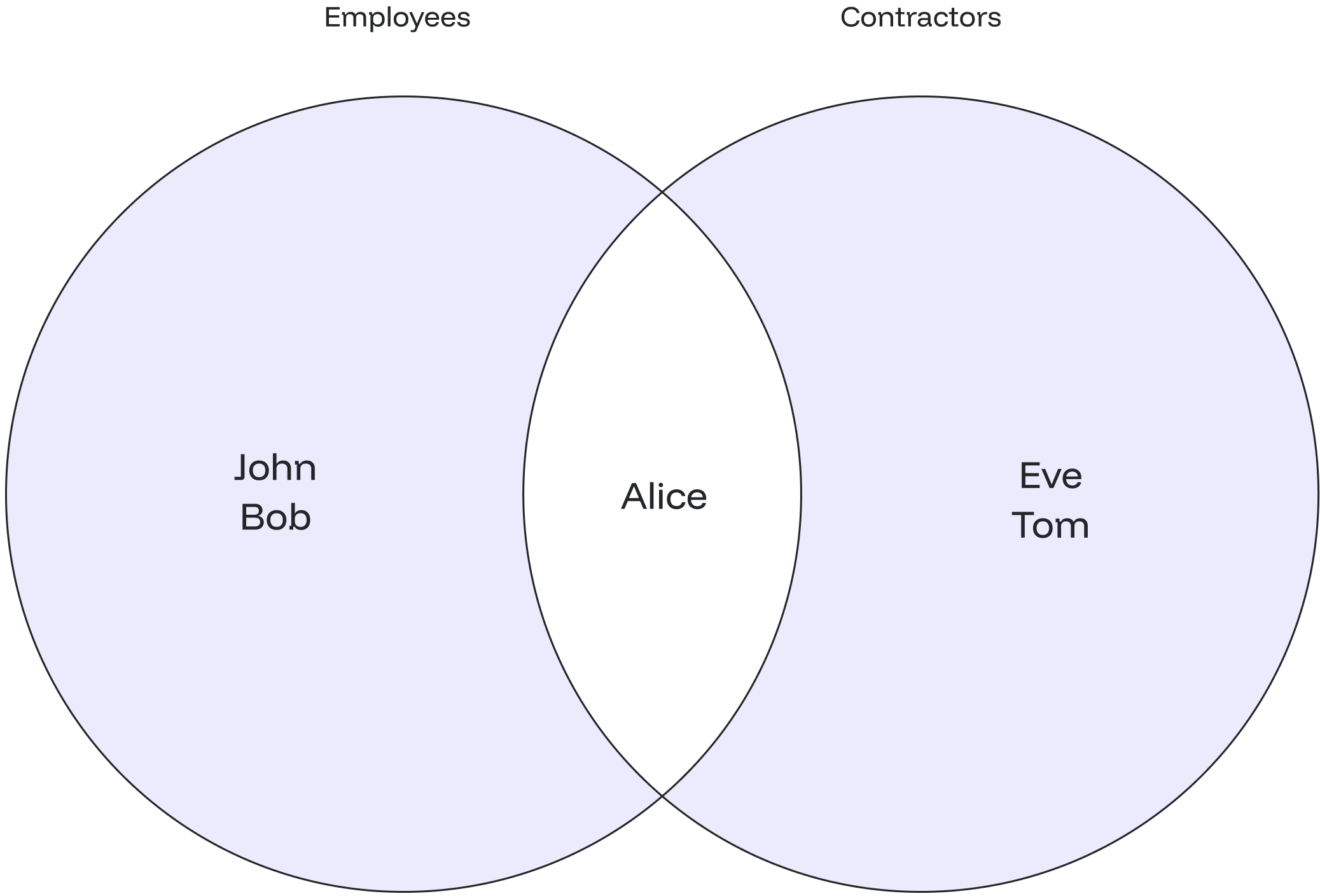
### Example Let's consider an example of the `UNION`. Assume we have a table called `employees` and another table called `contractors`. We want to retrieve a combined list of names from both tables, excluding duplicates: ```sql theme={null} CREATE TABLE employees ( emp_id INT, emp_name TEXT ); CREATE TABLE contractors ( contractor_id INT, contractor_name TEXT ); INSERT INTO employees VALUES (1, 'John'), (2, 'Alice'), (3, 'Bob'); INSERT INTO contractors VALUES (101, 'Alice'), (102, 'Eve'), (103, 'Tom'); ``` Verifying inserted values by using the `SELECT` statement: ```sql theme={null} SELECT * FROM employees; SELECT * FROM contractors; ``` ```sql theme={null} emp_id | emp_name --------+---------- 1 | John 2 | Alice 3 | Bob contractor_id | contractor_name ---------------+----------------- 101 | Alice 102 | Eve 103 | Tom ``` Let’s combine the values from the tables: ```sql theme={null} SELECT emp_name FROM employees UNION SELECT contractor_name FROM contractors; ``` You will get the values of both tables, and there won’t be any duplicate values. ```sql theme={null} emp_name ---------- Alice Bob Eve John Tom ``` The diagram below shows that the duplicate name "Alice" is represented only once in the output, fulfilling the requirement to avoid duplicate entries. ## UNION ALL ### Overview The `UNION ALL` combines the result sets of 2 or more select statements, returning all rows from the query and not removing duplicate rows between the tables. ### Syntax Below is the syntax of the `UNION ALL`: ```sql theme={null} SELECT value1, value2, ... value_n FROM tables UNION ALL SELECT value1, value2, ... value_n FROM tables; ``` The parameters from the syntax are explained below: * `value1, value2, ... value_n`: The columns you wish to retrieve. You can also retrieve all the values using the `SELECT * FROM` query. * `table1, table2`: The tables that you wish to retrieve records from. **Things to consider:**
1. The data types of corresponding columns in the `SELECT` queries must be compatible.
2. The order of columns is flexible as long as the columns in consecutive places are pairwise compatible.
### Example Suppose you have two separate tables, `sales_2022` and `sales_2023`, containing sales data for different years. You want to combine the sales data from both tables to get a complete list of sales transactions without removing duplicates. ```sql theme={null} CREATE TABLE sales_2022 ( transaction_id INT, product_name TEXT, sale_amount INT ); CREATE TABLE sales_2023 ( transaction_id INT, product_name TEXT, sale_amount INT ); INSERT INTO sales_2022 VALUES (1, 'Product A', 1000), (2, 'Product B', 500), (3, 'Product C', 750); INSERT INTO sales_2023 VALUES (4, 'Product A', 1200), (5, 'Product D', 800), (6, 'Product E', 950); ``` Verifying inserted values by using the `SELECT` statement: ```sql theme={null} SELECT * FROM sales_2022; SELECT * FROM sales_2023; ``` ```sql theme={null} transaction_id | product_name | sale_amount ----------------+--------------+------------- 1 | Product A | 1000 2 | Product B | 500 3 | Product C | 750 transaction_id | product_name | sale_amount ----------------+--------------+------------- 4 | Product A | 1200 5 | Product D | 800 6 | Product E | 950 ``` Let’s combine all values from the tables by using the `UNION ALL`: ```sql theme={null} SELECT product_name, sale_amount FROM sales_2022 UNION ALL SELECT product_name, sale_amount FROM sales_2023; ``` In this case, it will display all the values of the first table followed by all the contents of the second table. ```sql theme={null} product_name | sale_amount --------------+------------- Product A | 1000 Product B | 500 Product C | 750 Product A | 1200 Product D | 800 Product E | 950 ``` The diagram illustrates that with the `UNION ALL`, all values are displayed, including the duplicate ones. --- # 
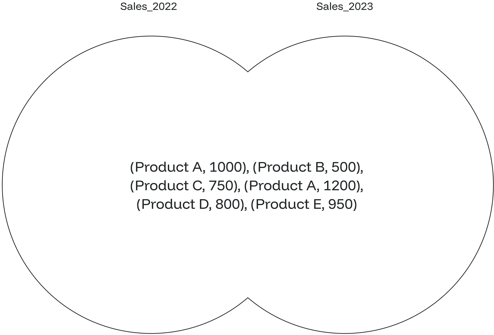
Source: https://docs.oxla.com/sql-reference/sql-functions/timestamp-functions/unix-macros.md > ## Documentation Index > Fetch the complete documentation index at: https://docs.oxla.com/llms.txt > Use this file to discover all available pages before exploring further. # UNIX_MICROS ## Overview The `UNIX_MICROS()` function returns a given timestamp into a UNIX timestamp in microseconds, from 1970-01-01 00:00:00-00 (can be negative). Its syntax is illustrated below: ```sql theme={null} SELECT UNIX_MICRO(TIMESTAMP) ``` Its input type is a TIMESTAMP expression, and the return data type is `BIGINT` representing time in microseconds. ## Examples ### Case #1: Basic `UNIX_MICROS()` function The below example uses the `UNIX_MICROS()` function to convert a given timestamp into a UNIX timestamp in microseconds: ```sql theme={null} SELECT UNIX_MICRO(TIMESTAMP "2022-12-25 13:30:00+00") AS unix_microsvalues; ``` The final output will be as follows: ```sql theme={null} +-----------------------------+ | unix_microsvalues | +-----------------------------+ | 1671975000000000.000000 | +-----------------------------+ ``` ### Case #2: `UNIX_MICROS()` function using columns Let’s suppose we have a table named **time\_example** with the following timestamp values: ```sql theme={null} CREATE TABLE time_example ( time_stamp timestamp ); INSERT INTO time_example VALUES ('2022-12-25 13:30:00'), ('2021-10-02 06:30:00'), ('2020-09-25 07:25:00'); ``` ```sql theme={null} SELECT * FROM time_example; ``` The above query will show the following table: ```sql theme={null} +-------------------------+ | time_example | +-------------------------+ | 2022-12-25 13:30:00 | | 2021-10-02 06:30:00 | | 2020-09-25 07:25:00 | +-------------------------+ ``` We want to convert all timestamp values into UNIX timestamp values in microseconds. To do that, we have to run the following query: ```sql theme={null} SELECT time_stamp, UNIX_MICROS(time_stamp) AS time_micros FROM time_example; ``` The output displays all the timestamp entries in the **time\_stamp** column and the converted UNIX timestamps in microseconds in the column **time\_micros**. ```sql theme={null} +-------------------------+--------------------------+ | time_stamp | time_micros | +-------------------------+--------------------------+ | 2022-12-25 13:30:00 | 1671975000000000.000000 | | 2021-10-02 06:30:00 | 1633156200000000.000000 | | 2020-09-25 07:25:00 | 1601018700000000.000000 | +-------------------------+--------------------------+ ``` --- # Source: https://docs.oxla.com/sql-reference/sql-functions/timestamp-functions/unix-micros.md > ## Documentation Index > Fetch the complete documentation index at: https://docs.oxla.com/llms.txt > Use this file to discover all available pages before exploring further. # UNIX_MICROS ## Overview The `UNIX_MICROS()` function returns a given timestamp into a UNIX timestamp in microseconds, from 1970-01-01 00:00:00-00 (can be negative). Its syntax is illustrated below: ```sql theme={null} SELECT UNIX_MICRO(TIMESTAMP) ``` Its input type is a TIMESTAMP expression, and the return data type is `int64` representing time in microseconds. ## Examples ### Case #1: Basic `UNIX_MICROS()` function The below example uses the `UNIX_MICROS()` function to convert a given timestamp into a UNIX timestamp in microseconds: ```sql theme={null} SELECT UNIX_MICRO(TIMESTAMP "2022-12-25 13:30:00+00") AS unix_microsvalues; ``` The final output will be as follows: ```sql theme={null} +-----------------------------+ | unix_microsvalues | +-----------------------------+ | 1671975000000000.000000 | +-----------------------------+ ``` ### Case #2: `UNIX_MICROS()` function using columns Let’s suppose we have a table named **time\_example** with the following timestamp values: ```sql theme={null} CREATE TABLE time_example ( time_stamp timestamp ); INSERT INTO time_example VALUES ('2022-12-25 13:30:00'), ('2021-10-02 06:30:00'), ('2020-09-25 07:25:00'); ``` ```sql theme={null} SELECT * FROM time_example; ``` The above query will show the following table: ```sql theme={null} +-------------------------+ | time_example | +-------------------------+ | 2022-12-25 13:30:00 | | 2021-10-02 06:30:00 | | 2020-09-25 07:25:00 | +-------------------------+ ``` We want to convert all timestamp values into UNIX timestamp values in microseconds. To do that, we have to run the following query: ```sql theme={null} SELECT time_stamp, UNIX_MICROS(time_stamp) AS time_micros FROM time_example; ``` The output displays all the timestamp entries in the **time\_stamp** column and the converted UNIX timestamps in microseconds in the column **time\_micros**. ```sql theme={null} +-------------------------+--------------------------+ | time_stamp | time_micros | +-------------------------+--------------------------+ | 2022-12-25 13:30:00 | 1671975000000000.000000 | | 2021-10-02 06:30:00 | 1633156200000000.000000 | | 2020-09-25 07:25:00 | 1601018700000000.000000 | +-------------------------+--------------------------+ ``` --- # Source: https://docs.oxla.com/sql-reference/sql-functions/timestamp-functions/unix-millis.md > ## Documentation Index > Fetch the complete documentation index at: https://docs.oxla.com/llms.txt > Use this file to discover all available pages before exploring further. # UNIX_MILLIS ## Overview The `UNIX_MILLIS()` function returns a given timestamp to a UNIX timestamp in milliseconds from 1970-01-01 00:00:00-00 (can be negative). Its syntax is illustrated below: ```sql theme={null} SELECT UNIX_MILLIS(TIMESTAMP) ``` Its input type is a TIMESTAMP expression, and the return data type is `BIGINT` representing time in milliseconds. ## Examples ### Case #1: Basic `UNIX_MILLIS()` function The below example uses the `UNIX_MILLIS()` function to convert a given timestamp into a UNIX timestamp in milliseconds: ```sql theme={null} SELECT UNIX_MILLIS(TIMESTAMP "1996-5-02 7:15:00+00") AS unix_millisvalues; ``` The final output will be as follows: ```sql theme={null} +-----------------------------+ | unix_millisvalues | +-----------------------------+ | 831021300000.000000 | +-----------------------------+ ``` ### Case #2: `UNIX_MILLIS()` function using columns Let’s suppose we have a table named **time\_example **with the following timestamp values in the** time\_stamp** column: ```sql theme={null} CREATE TABLE time_example ( time_stamp timestamp ); INSERT INTO time_example VALUES ('2004-07-23 11:30:00+00'), ('2011-02-12 04:45:00+00'), ('1975-08-03 07:50:00+00'); ``` ```sql theme={null} SELECT * FROM time_example; ``` The above query will show the following table: ```sql theme={null} +-------------------------+ | time_example | +-------------------------+ | 2004-07-23 11:30:00 | | 2011-02-12 04:45:00 | | 1975-08-03 07:50:00 | +-------------------------+ ``` We want to convert all timestamp values into UNIX timestamp values in milliseconds. To do that, we have to run the following query: ```sql theme={null} SELECT time_stamp, UNIX_MILLIS(time_stamp) AS time_millis FROM time_example; ``` The output displays all the timestamp entries of the table in the \*\*time\_stamp \*\*column and the converted UNIX milliseconds timestamp entries in the column **time\_millis**. ```sql theme={null} +-------------------------+-----------------------+ | time_stamp | time_millis | +-------------------------+-----------------------+ | 2004-07-23 11:30:00 | 1090582200000.000000 | | 2011-02-12 04:45:00 | 1297485900000.000000 | | 1975-08-03 07:50:00 | 176284200000.000000 | +-------------------------+-----------------------+ ``` --- # Source: https://docs.oxla.com/sql-reference/sql-functions/timestamp-functions/unix-seconds.md > ## Documentation Index > Fetch the complete documentation index at: https://docs.oxla.com/llms.txt > Use this file to discover all available pages before exploring further. # UNIX_SECONDS ## Overview The `UNIX_SECONDS()` function returns a given timestamp to a UNIX timestamp in seconds, from 1970-01-01 00:00:00-00. Its syntax is illustrated below: ```sql theme={null} SELECT UNIX_SECONDS(TIMESTAMP) ``` Its input type is a TIMESTAMP expression, and the return data type is `BIGINT` representing time in seconds. ## Examples ### Case #1: Basic `UNIX_SECONDS()` function The below example uses the `UNIX_SECONDS()` function to convert a given timestamp into a UNIX timestamp in seconds: ```sql theme={null} SELECT UNIX_SECONDS(TIMESTAMP "2008-12-25 15:30:00+00") AS unix_secondsvalues; ``` The final output will be as follows: ```sql theme={null} +-----------------------------+ | unix_secondsvalues | +-----------------------------+ | 1230219000.000000 | +-----------------------------+ ``` ### Case #2: `UNIX_SECONDS()` function using columns Let’s suppose we have a table named \*\*time\_example \*\*with the following timestamp values in the **time\_stampvalues** column: ```sql theme={null} CREATE TABLE time_example ( time_stampvalues timestamp ); INSERT INTO time_example VALUES ('2022-12-25 13:30:00'), ('2020-09-25 07:25:00'), ('2008-12-25 15:30:00'), ('2021-10-02 06:30:00'); ``` ```sql theme={null} SELECT * FROM time_example; ``` The above query will return the following table: ```sql theme={null} +-------------------------+ | time_stampvalues | +-------------------------+ | 2022-12-25 13:30:00 | | 2020-09-25 07:25:00 | | 2008-12-25 15:30:00 | | 2021-10-02 06:30:00 | +-------------------------+ ``` 1. We want to convert all timestamp values into UNIX timestamp values in seconds. To do that, we have to run the following query: ```sql theme={null} SELECT time_stampvalues, UNIX_SECONDS(time_stampvalues) AS time_secondsvalues FROM time_example; ``` 2. The output displays all the timestamp entries of the table in the **time\_stampvalues** column and the converted UNIX seconds timestamp entries in the column **time\_secondsvalues**. ```sql theme={null} +-------------------------+-----------------------+ | time_stampvalues | time_secondsvalues | +-------------------------+-----------------------+ | 2022-12-25 13:30:00 | 1671975000.000000 | | 2020-09-25 07:25:00 | 1601018700.000000 | | 2008-12-25 15:30:00 | 1230219000.000000 | | 2021-10-02 06:30:00 | 1633156200.000000 | +-------------------------+-----------------------+ ``` --- # Source: https://docs.oxla.com/sql-reference/sql-mutations/update.md > ## Documentation Index > Fetch the complete documentation index at: https://docs.oxla.com/llms.txt > Use this file to discover all available pages before exploring further. # UPDATE ## **Overview** The `UPDATE` mutation is used to modify the existing records in a table. This support has limitations: * Only **one data mutation (DELETE or UPDATE)** at given moment is possible, trying to run another one will result in failure. * Data mutations rewrite all files containing the data from the UPDATE/DELETE condition. Please note that running `DELETE from table` without any condition is possible, but it will be much slower than just `DROP TABLE table`. * The syntax is simplified in comparison to Postgres. For example, the `SET column=` operation doesn’t support sub-SELECT as the value, also the `WHERE` clause cannot contain sub-SELECT. **Feature Update: Initial Release**.
This marks the initial release of our new Mutation feature, providing you with the ability to update data. The Mutations involve rewriting entire files which take several minutes and could generate infrastructure costs. We are aiming to enhance and optimize this feature in future updates!
## Syntax The syntax for `UPDATE` mutation is as follows: ```sql theme={null} UPDATE table SET column1 = expression1, column2 = expression2 ... WHERE conditions; ``` In this syntax: * `table`: The name of the table you want to update. * `column1, column2`: The columns that you wish to update. * `expression1, expression2`: The new values to assign to column1, column2, and so on. Each column is set to its corresponding expression. * `WHERE conditions` **(Optional)**: The conditions that must be met for the update to execute. If no conditions are provided, all table records will be updated. ## Examples Let's create a sample table called tasks: ```sql theme={null} CREATE TABLE tasks ( task_id INT, task_name TEXT, status TEXT ); INSERT INTO tasks (task_id, task_name, status) VALUES (1001, 'Task A', 'pending'), (1002, 'Task B', 'in-progress'), (1003, 'Task C', 'pending'); ``` The tasks table will be created as shown below: ```sql theme={null} task_id | task_name | status ---------+-----------+------------- 1001 | Task A | pending 1002 | Task B | in-progress 1003 | Task C | pending ``` Now, let's see the following cases for updating the table: ### Case #1: Update a Single Column 1. In this case, we want to update the `status` column to “completed” for the record where `task_id` is 1001. ```sql theme={null} UPDATE tasks SET status = 'completed' WHERE task_id = 1001; ``` 2. The output below shows that the update was successful. ```sql theme={null} UPDATE ``` 3. Check the updated table by running the `SELECT` query below: ```sql theme={null} SELECT * FROM tasks; ``` 4. The `UPDATE` mutation updates the status to “completed” for the task with ID 1001. ```sql theme={null} task_id | task_name | status ---------+-----------+------------- 1001 | Task A | completed 1002 | Task B | in-progress 1003 | Task C | pending ``` ### Case #2: Update Multiple Columns 1. Let’s assume we want to update the `task_name` and `status` columns for the record where `task_id` is 1002. ```sql theme={null} UPDATE tasks SET task_name = 'Updated Task B', status = 'completed' WHERE task_id = 1002; ``` 2. The output below shows that the update was successful. ```sql theme={null} UPDATE ``` 3. Check the updated table by running the `SELECT` query below: ```sql theme={null} SELECT * FROM tasks; ``` 4. Here, the task name and status columns are updated for the task with ID 1002. ```sql theme={null} task_id | task_name | status ---------+----------------+----------- 1001 | Task A | completed 1002 | Updated Task B | completed 1003 | Task C | pending ``` --- # Source: https://docs.oxla.com/sql-reference/sql-functions/string-functions/upper.md > ## Documentation Index > Fetch the complete documentation index at: https://docs.oxla.com/llms.txt > Use this file to discover all available pages before exploring further. # UPPER ## Overview The `UPPER()` function returns a given string, an expression, or values in a column in all uppercase letters. The syntax of the function is illustrated below: ```sql theme={null} UPPER(string) ``` It accepts input as a string and returns text in uppercase letters. **Special Case:** * If characters in the input are not of type string, they remain unaffected by the `UPPER()` function. * We support Unicode for the `UPPER()` function. ## Examples ### #Case 1: Basic `UPPER()` function The following basic query converts the given string in all uppercase alphabets: ```sql theme={null} SELECT UPPER('PostGreSQL'); ``` The final output will be as follows: ```sql theme={null} +-------------+ | upper | +-------------+ | POSTGRESQL | +-------------+ ``` ### Case 2: UPPER() function using columns and CONCAT() function Let’s see how the `UPPER()` function works using an example with columns. We have a table named **personal\_details** containing employee's **id**, **first\_name**, **last\_name**, and **gender** of a retail store: ```sql theme={null} CREATE TABLE personal_details ( id int, first_name text, last_name text, gender text ); INSERT INTO personal_details (id, first_name, last_name, gender) VALUES (1,'Mark','Wheeler','M'), (2,'Tom','Hanks','M'), (3,'Jane','Hopper','F'), (4,'Emily','Byers','F'), (5,'Lucas','Sinclair','M'); ``` ```sql theme={null} SELECT * FROM personal_details; ``` The above query will show the following table: ```sql theme={null} +-----+-------------+-------------+----------+ | id | first_name | last_name | gender | +-----+-------------+-------------+----------+ | 1 | Mark | Wheeler | M | | 2 | Tom | Hanks | M | | 3 | Jane | Hopper | F | | 4 | Emily | Byers | F | | 5 | Lucas | Sinclair | M | +-----+-------------+-------------+----------+ ``` Let’s assume that: 1. We want to convert employees' first and last names with **id** numbers 1, 3, and 5 to all uppercase letters. 2. Then, combine them using the `CONCAT()` function into one **full\_name** column in uppercase. It can be done using the following query: ```sql theme={null} SELECT CONCAT (UPPER(first_name),' ', UPPER(last_name)) as full_name FROM personal_details where id in (1, 3, 5); ``` The output displays the first and last names of employees with the specified ids in uppercase letters: ```sql theme={null} +---------------------+ | full_name | +---------------------+ | MARK WHEELER | | JANE HOPPER | | LUCAS SINCLAIR | +---------------------+ ``` --- # Source: https://docs.oxla.com/sql-reference/sql-functions/aggregate-functions/var-pop.md > ## Documentation Index > Fetch the complete documentation index at: https://docs.oxla.com/llms.txt > Use this file to discover all available pages before exploring further. # VAR_POP() ## Overview The `VAR_POP()` aggregate function calculates the population variance of a set of numeric values. ## Syntax The syntax for this function is as follows: ```sql theme={null} VAR_POP(expression) ``` ## Parameters * `expression`: numeric expression or column for which the population variance is calculated ## Example For the needs of this section we're going to use a simplified version of the `film` table from the Pagila database, containing only the `title`, `length` and `rating` columns. The complete schema for the `film` table can be found on the Pagila database website. ```sql theme={null} DROP TABLE IF EXISTS film; CREATE TABLE film ( title text NOT NULL, length int, rating int ); INSERT INTO film(title, length, rating) VALUES ('ATTRACTION NEWTON', 83, 5), ('CHRISTMAS MOONSHINE', 150, 7), ('DANGEROUS UPTOWN', 121, 4), ('KILL BROTHERHOOD', 54, 3), ('HALLOWEEN NUTS', 47, 5), ('HOURS RAGE', 122, 7), ('PIANIST OUTFIELD', 136, 7), ('PICKUP DRIVING', 77, 3), ('INDEPENDENCE HOTEL', 157, 7), ('PRIVATE DROP', 106, 4), ('SAINTS BRIDE', 125, 3), ('FOREVER CANDIDATE', 131, 7), ('MILLION ACE', 142, 5), ('SLEEPY JAPANESE', 137, 4), ('WRATH MILE', 176, 7), ('YOUTH KICK', 179, 7), ('CLOCKWORK PARADISE', 143, 5); ``` The query below uses the `VAR_POP()` function to calculate the population variance for the `length` column: ```sql theme={null} SELECT VAR_POP(length) AS LengthPopulationVariance FROM film; ``` By executing the above query, we will get the following output: ```sql theme={null} lengthpopulationvariance -------------------------- 1386.442906574394 (1 row) ``` --- # Source: https://docs.oxla.com/sql-reference/sql-functions/aggregate-functions/var-samp.md > ## Documentation Index > Fetch the complete documentation index at: https://docs.oxla.com/llms.txt > Use this file to discover all available pages before exploring further. # VAR_SAMP() ## Overview The `VAR_SAMP()` aggregate function calculates the sample variance of a set of numeric values. This function measures the spread of data points around the mean, assuming the data is a sample of a larger population. ## Syntax The syntax for this function is as follows: ```sql theme={null} VAR_SAMP(expression) ``` ## Parameters * `expression`: numeric expression or column for which the sample variance is calculated ## Example For the needs of this section we're going to use a simplified version of the `film` table from the Pagila database, containing only the `title`, `length` and `rating` columns. The complete schema for the `film` table can be found on the Pagila database website. ```sql theme={null} DROP TABLE IF EXISTS film; CREATE TABLE film ( title text NOT NULL, length int, rating int ); INSERT INTO film(title, length, rating) VALUES ('ATTRACTION NEWTON', 83, 5), ('CHRISTMAS MOONSHINE', 150, 7), ('DANGEROUS UPTOWN', 121, 4), ('KILL BROTHERHOOD', 54, 3), ('HALLOWEEN NUTS', 47, 5), ('HOURS RAGE', 122, 7), ('PIANIST OUTFIELD', 136, 7), ('PICKUP DRIVING', 77, 3), ('INDEPENDENCE HOTEL', 157, 7), ('PRIVATE DROP', 106, 4), ('SAINTS BRIDE', 125, 3), ('FOREVER CANDIDATE', 131, 7), ('MILLION ACE', 142, 5), ('SLEEPY JAPANESE', 137, 4), ('WRATH MILE', 176, 7), ('YOUTH KICK', 179, 7), ('CLOCKWORK PARADISE', 143, 5); ``` They query below uses the `VAR_SAMP()` function to calculate the sample variance for the `length` column where `rating` is greater than or equal to 4: ```sql theme={null} SELECT VAR_SAMP(length) AS LengthSampleVariance FROM film WHERE rating >= 4; ``` By running the above code, we will get the following output: ```sql theme={null} lengthsamplevariance ---------------------- 1219.7582417582407 (1 row) ``` --- # Source: https://docs.oxla.com/sql-reference/sql-functions/aggregate-functions/variance.md > ## Documentation Index > Fetch the complete documentation index at: https://docs.oxla.com/llms.txt > Use this file to discover all available pages before exploring further. # VARIANCE() ## Overview The `VARIANCE()` aggregate function calculate the sample variance of a set of numeric values. Variance measures the spread of data points around the mean, providing insight into how much the values deviate from the average. ## Syntax The syntax for this function is as follows: ```sql theme={null} VARIANCE(expression) ``` ## Parameters * `expression`: numeric expression or column for which the variance is calculated ## Example For the needs of this section, we're going to use a simplified version of the `film` table from the Pagila database, containing only the `title`, `length` and `rating` columns. The complete schema for the `film` table can be found on the Pagila database website. ```sql theme={null} DROP TABLE IF EXISTS film; CREATE TABLE film ( title text NOT NULL, length int, rating int ); INSERT INTO film(title, length, rating) VALUES ('ATTRACTION NEWTON', 83, 5), ('CHRISTMAS MOONSHINE', 150, 7), ('DANGEROUS UPTOWN', 121, 4), ('KILL BROTHERHOOD', 54, 3), ('HALLOWEEN NUTS', 47, 5), ('HOURS RAGE', 122, 7), ('PIANIST OUTFIELD', 136, 7), ('PICKUP DRIVING', 77, 3), ('INDEPENDENCE HOTEL', 157, 7), ('PRIVATE DROP', 106, 4), ('SAINTS BRIDE', 125, 3), ('FOREVER CANDIDATE', 131, 7), ('MILLION ACE', 142, 5), ('SLEEPY JAPANESE', 137, 4), ('WRATH MILE', 176, 7), ('YOUTH KICK', 179, 7), ('CLOCKWORK PARADISE', 143, 5); ``` The query below uses the `VARIANCE()` function to calculate the variance for the `length` column: ```sql theme={null} SELECT VARIANCE(length) AS LengthVariance FROM film; ``` By executing the code above, we will get the following output: ```sql theme={null} lengthvariance -------------------- 1473.0955882352937 (1 row) ``` --- # Source: https://docs.oxla.com/welcome.md > ## Documentation Index > Fetch the complete documentation index at: https://docs.oxla.com/llms.txt > Use this file to discover all available pages before exploring further. # Welcome > Discover everything you need to know about Oxla right here, right now! Hero Light Hero Dark } href="/sql-reference/overview" className="max-w-xs mx-auto" > Learn about SQL functions, statements, clauses and data types that Oxla supports --- # Source: https://docs.oxla.com/introduction/what-is-oxla-and-why-use-it.md > ## Documentation Index > Fetch the complete documentation index at: https://docs.oxla.com/llms.txt > Use this file to discover all available pages before exploring further. # What is Oxla and why use it Oxla is a highly resource-efficient, self-hosted, column-oriented OLAP database and query engine. It’s available under a proprietary license with [capacity-based pricing](https://www.oxla.com/pricing), and also comes in a forever-free, single-node [Developer Edition](/quickstart) for POCs and non-commercial use. ## Key Characteristics ### Vectorized Query Execution Oxla uses a massively parallel processing (MPP) architecture at the core of its compute engine for high-performance processing. While MPP has been the standard in analytics systems for over a decade, Oxla takes a modern approach: it’s a new system built from the ground up, without relying on third-party components. This clean-slate design lets us apply recent advancements in computer science to a fresh codebase, with a focus on [low-level optimizations that improve resource efficiency](#optimized-data-transfer-between-cpu-and-ram), both in the query engine and across the system. ### Columnar Storage Optimization Transactional (OLTP) databases like PostgreSQL or MS SQL Server use a row-oriented design, optimized for high-frequency writes. Columnar storage, by contrast, is designed for analytical workloads, allowing for faster scans, better compression, and more efficient aggregations. Oxla supports high-speed ingestion of .csv, ORC, Parquet, and JSON files. For example, you can easily feed large volumes of transactional data from OLTP sources into Oxla at scale. ### Decoupled Storage & Compute While Oxla isn’t currently capable of querying external data in place at the source (though this is a high-priority item on our immediate [roadmap](/product-roadmap)), it benefits from a decoupled storage & compute architecture. This means compute resources can be scaled independently of storage, allowing for more efficient resource allocation, easier deployment, and better cost control. ### Efficient Data Compression Depending on the structure and contents of the data, Oxla achieves up to 95% compression. This enables cost-effective long-term storage, and the ultra-efficient query engine supports fast historical analytics over large datasets (up to 400 terabytes). ### Distributed, Multi-node Architecture Oxla is a distributed database, meaning it can run across multiple CPUs (nodes) in parallel for horizontal scaling, characteristic of cloud-native systems. Adaptive query pipelines efficiently handle all types of operations across nodes. At the same time, thanks to its unique resource efficiency, Oxla delivers strong performance even in single-node deployments and can scale vertically by adding more CPU cores. Execution strategies are selected at runtime based on workload characteristics, ensuring optimal performance in both single-node and multi-node setups. ### SQL Support Like many modern OLAP systems, Oxla uses its own declarative query language under the hood, but provides [SQL support](/sql-reference/overview) to users. Oxla aims for close compatibility with PostgreSQL, including support for core SQL constructs such as `FROM`, `JOIN`, `GROUP BY`, `ORDER BY`, and window functions. ### Optimized Data Transfer Between CPU and RAM Over the past decade, CPUs have scaled from 4–8 cores to over 100, but memory bandwidth hasn’t kept pace. This hardware limitation creates a critical bottleneck for analytical compute engines. Oxla introduces a set of low-level memory access and caching optimizations to address this issue and achieve high resource efficiency. * **Compressed data** reduces the volume transferred between storage, memory, and CPU * **User-space storage caches** minimize overhead from kernel-level memory operations * **A custom data format** enhances data locality * **Hybrid row/column formats** allow better alignment with CPU cache lines and vectorized execution * **Temporal access patterns** help retain frequently used data in memory longer, reducing cache misses ## Why choose Oxla ### Scalability through resource-efficiency A common reason to move to a fully-managed cloud data warehouse is the promise of “infinite scalability,” made possible by on-demand infrastructure in the cloud. At Oxla, we believe systems should scale through smarter, more efficient use of hardware—not by simply throwing more resources at the problem. This principle is baked into how Oxla is designed and built. By maximizing resource efficiency, Oxla lets you continue self-hosting your data warehouse while handling growing datasets. This approach reduces total cost of ownership by squeezing more out of your existing infra, helping you delay expensive upgrades and maximize ROI. ### Straightforward self-hosting Oxla runs on x86-64 CPUs (Intel/AMD/ARM) and is deployed via Docker on Linux, accessed through PostgreSQL Client 14. The same Docker image can be run in a traditional client-server setup (either single-node or multi-node) or locally. Oxla’s [configuration file](/configuration-deployment/configuration/oxla-configuration-file) is designed with simplicity in mind. It employs a streamlined, human-readable YAML format that covers essential settings without the verbosity or complexity seen in some other systems. This way, Oxla is simple to integrate into existing environments with minimal operational overhead. ### Unified support for batch, low-latency, time-series, and multi-dimensional analytics Oxla supports a wide range of analytical workloads in a single system. You can power real-time BI dashboards, process log data, run time-series analytics, and perform exploratory queries over terabyte-scale datasets without switching tools or maintaining separate systems. Combined with scalable and easy-to-manage self-hosting, this makes Oxla particularly suitable for unified analytics in critical infrastructure such as the telco, energy, and defense sectors. --- # Source: https://docs.oxla.com/sql-reference/sql-clauses/where.md > ## Documentation Index > Fetch the complete documentation index at: https://docs.oxla.com/llms.txt > Use this file to discover all available pages before exploring further. # WHERE ## Overview The `WHERE` clause returns a specific value from a table or multiple tables based on specified conditions. It will filter out records you do not want to be included and only returns the exact result when the condition is fulfilled. ## Syntax The basic syntax of the WHERE clause is as follows − ```sql theme={null} SELECT column1, column2, ... FROM table_name WHERE [condition] ``` Let’s explore the above syntax: * `SELECT column1, column2, ...` defines the columns where the records will be displayed. * `FROM table_name` sets the table name where the records will be taken from. * `WHERE [condition]`specifies the search condition using comparison or logical operators (e.g., `>`, `=`, `LIKE`) It starts with the `FROM` clause **->** then it executes the `WHERE` condition **->** after that, it will `SELECT` the specified columns. ## Examples Let’s assume that we have a table salary with records as follows: ```sql theme={null} CREATE TABLE salary ( empid int, empname text, empdept text, empaddress text, empsalary int ); INSERT INTO salary (empid, empname, empdept, empaddress, empsalary) VALUES (2001,'Paul','HR', 'California', null ), (2002,'Brandon','Product', 'Norway', 15000), (2003,'Bradley','Marketing', 'Texas', null), (2004,'Lisa','Marketing', 'Houston', 10000), (2005,'Emily','Marketing', 'Texas', 20000), (2006,'Bobby','Finance', 'Seattle', 20000), (2007,'Parker','Project', 'Texas', 45000); ``` ```sql theme={null} SELECT * FROM salary; ``` It will create a table as shown below: ```sql theme={null} +--------+-----------+------------+-------------+------------+ | empid | empname | empdept | empaddress | empsalary | +--------+-----------+------------+-------------+------------+ | 2001 | Paul | HR | California | null | | 2002 | Brandon | Product | Norway | 15000 | | 2003 | Bradley | Marketing | Texas | null | | 2004 | Lisa | Marketing | Houston | 10000 | | 2005 | Emily | Marketing | Texas | 20000 | | 2006 | Bobby | Finance | Seattle | 20000 | | 2007 | Parker | Project | Texas | 45000 | +--------+-----------+------------+-------------+------------+ ``` ### #Case 1: WHERE clause with `=` Operator Here we will be using the “equal” operator to look up the employee who works in the Marketing department: ```sql theme={null} SELECT empname, empdept FROM salary WHERE empdept = 'Marketing'; ``` The above command will create the following result: ```sql theme={null} +------------+-------------+ | empname | empdept | +------------+-------------+ | Bradley | Marketing | | Emily | Marketing | | Lisa | Marketing | +------------+-------------+ ``` The value defined in the `WHERE` clause’s condition is **case-sensitive**, so ensure that you specify the correct and precise value. ### #Case 2: WHERE clause with `!=` Operator Here we will be using the “not equal” operator to look up the employee who doesn’t live in Texas: ```sql theme={null} SELECT empname, empdept, empaddress FROM salary WHERE empaddress != 'Texas'; ``` We can use the `<>` operator for another “not equal” operator. The above query will give the following result: ```sql theme={null} +------------+------------+--------------+ | empname | empdept | empaddress | +------------+------------+--------------+ | Paul | HR | California | | Brandon | Product | Norway | | Lisa | Marketing | Houston | | Bobby | Finance | Seattle | +------------+------------+--------------+ ``` The value defined in the `WHERE` clause's condition is **case-sensitive**. If you set `texas` it will return all records from the salary table. ### #Case 3: WHERE clause with `>` Operator Here we will be using the “greater than” operator to figure out who has a salary above 20000: ```sql theme={null} SELECT empname, empdept, empsalary FROM salary WHERE empsalary > 20000; ``` We can use the `<` operator for a “less than” condition. The output will let us know that Parker has a salary greater than 20000: ```sql theme={null} +------------+------------+-------------+ | empname | empdept | empsalary | +------------+------------+-------------+ | Parker | Project | 45000 | +------------+------------+-------------+ ``` ### #Case 4: WHERE clause with `<=` Operator Here we will be using the “less than or equal to” operator to see who has a salary less than or equal to 15000: ```sql theme={null} SELECT empname, empdept, empsalary FROM salary WHERE empsalary <= '15000'; ``` We can use the `>=` operator for a “greater than or equal to” condition. The output will let us know that Brandon has a salary equal to 15000 and Lisa has a salary of less than 15000: ```sql theme={null} +------------+------------+-------------+ | empname | empdept | empsalary | +------------+------------+-------------+ | Brandon | Product | 15000 | | Lisa | Marketing | 10000 | +------------+------------+-------------+ ``` ### #Case 5: WHERE clause with `LIKE` Operator Here we will use the “like” operator to retrieve the employee whose first name starts with **Br**. ```sql theme={null} SELECT * FROM salary WHERE empname LIKE 'Br%'; ``` Do the reverse to get the result based on the last string, `%string`. We will get an output where the above query fetches **Br**andon & **Br**adley. ```sql theme={null} +---------+------------+--------------+--------------+-----------+ | empid | empname | empdept | empaddress | empsalary | +---------+------------+-------------+--------------+------------+ | 2002 | Brandon | Product | Norway | null | | 2003 | Bradley | Marketing | Texas | 45000 | +---------+------------+-------------+--------------+------------+ ``` ### #Case 6: WHERE clause with `IS NULL` Operator Here we will use the “is null” operator to search for the employee who doesn’t have a salary value. It will return `true` and display the result set if a value is `NULL`; otherwise, it will return `false` with no result set. ```sql theme={null} SELECT * FROM salary WHERE empsalary IS NULL; ``` The above command will create the following result: ```sql theme={null} +---------+------------+-------------+--------------+------------+ | empid | empname | empdept | empaddress | empsalary | +---------+------------+-------------+--------------+------------+ | 2001 | Paul | HR | California | null | | 2003 | Brandon | Product | Norway | null | +---------+------------+-------------+--------------+------------+ ``` --- # Source: https://docs.oxla.com/sql-reference/sql-clauses/with.md > ## Documentation Index > Fetch the complete documentation index at: https://docs.oxla.com/llms.txt > Use this file to discover all available pages before exploring further. # WITH ## Overview The `WITH` clause provides a way to define auxiliary statements (referred by their alias names), that can be used within a more complex query sets. They are also known as Common Table Expressions (CTEs). ## Syntax The `WITH` clause precedes the primary statement it is attached to and contains a list of auxiliary statements with corresponding aliases. ```sql theme={null} WITH [with_statement_alias AS (with_statement_body)]+ primary_statement; ``` * **`primary_statement`**: has to be one of the following: `SELECT`, `INSERT`, `UPDATE`, `DELETE` * **`with_statement_body`**: has to be a `SELECT` statement (it can refer to aliases defined earlier in the query) ## Semantic Currently, Oxla only supports not materialised CTEs (e.g. each auxiliary query alias is replaced with its corresponding body at the early stages of the query processing). The following query: ```sql theme={null} WITH a AS (SELECT 77), b AS (SELECT * FROM a) SELECT * FROM b ``` is effectively turned into: ```sql theme={null} SELECT * FROM (SELECT * FROM (SELECT 77) AS a) AS b ``` Used auxiliary query gets the same alias (`AS b` part) as in the `WITH` clause. It can be changed by explicitly setting a new alias upon usage. ```sql theme={null} WITH b AS (SELECT 1 AS c1) SELECT b.c1, b1.c1 FROM b CROSS JOIN b AS b1; ``` ## Usage Not materialised `WITH` clauses are useful when you want to refactor some complex query to make it more readable. You can extract subqueries or even reuse them in several places, having only one definition. Thanks to code insertion, each use of a query will be optimized separately, specifically for the usage of its results by the parent query. For example: ```sql theme={null} WITH math_grades AS (SELECT g_date, semester_id, grade FROM grades WHERE subject="Math") SELECT * FROM (SELECT AVG(grade) FROM math_grades WHERE semester_id=2137) AS avg_semester_grades, (SELECT AVG(grade) FROM math_grades WHERE g_date >= (CURRENT_TIMESTAMP() - INTERVAL '1 y')) AS avg_year_grades ``` Both subqueries use the same auxiliary `math_grades` query, but each of them filters it using different keys. This way, both scans will only read a part of the table. If materialized CTE was used (which we don't support yet), the query engine would need to scan the whole table first and then filter the result twice, for each subquery. ## Alias Context You can't create more than one CTE with the same alias within a single `WITH` clause. However, if you create nested `SELECT` statements, each of them can have their own `WITH` clauses, creating their own contexts for defined aliases. The same alias can be defined in more than one context ```sql theme={null} WITH a AS ( # <-- creates context 1 SELECT 1 ) SELECT * FROM ( WITH a AS (SELECT 2) # <-- creates context 2 SELECT * FROM a # <-- uses context 2 ) CROSS JOIN a; # <-- uses context 1 ``` By executing the query above, you will receive `2, 1` as an output. When referencing an alias we use the context, which was defined at the nested query level. If it does not define the referenced alias, we move up one level and repeat searching for an alias definition. ```pgsql theme={null} WITH a AS ( SELECT 1 ) SELECT * FROM ( WITH b as (SELECT 2) SELECT * FROM b ) CROSS JOIN b; # <-- error ``` That query returns `ERROR: relation "b" does not exist`, as `b` is not defined in this context or any of the above.